-
Digital images are composed of pixels
-
Each pixel has a numeric value, often related to detected light
-
The same pixel values can be displayed in different ways
-
In scientific image processing, image appearance can be changed independently of pixel values by modifying a lookup table
Images & pixels
Chapter outline
Introduction
The smallest units from which an image is composed are its pixels.
The word 'pixel' is derived from picture element and, as far as the computer is concerned, each pixel is just a number.
When the image data is displayed, the values of pixels are usually converted into squares of particular colors – but this is only for our benefit to allow us to get a fast impression of the image contents, i.e. the approximate values of pixels and where they are in relation to one another.
When it comes to processing and analysis, we need to get past the display and delve into the real data: the numbers.
This distinction between data (the pixel values) and display (the colored squares) is particularly important in fluorescence microscopy. The pixels given to us by the microscope are measurements of the light being emitted by a sample. From these we can make deductions, e.g. more light may indicate the presence of a particular structure or substance, and knowing the exact values allows us to make comparisons and quantitative measurements. On the other hand, the colored squares do not matter for measurements: they are just nice to look at (Figure 1).
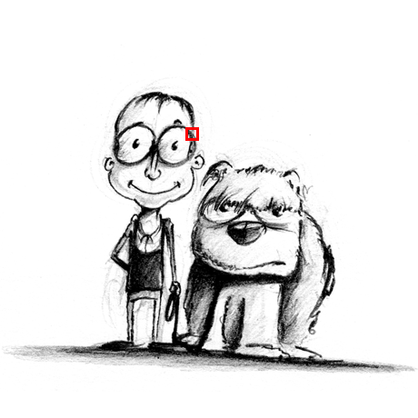
A: Original image
|

B: Enlarged view from (A)
|
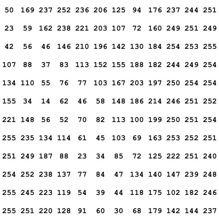
C: Pixel values of (B)
|
Figure 1: An image depicting an interestingly-matched couple I saw when walking home from work around the time of writing. (A) & (B) The image is shown using small squares of different shades of gray, where each square corresponds to a single pixel. This is only a convention used for display; the pixels themselves are stored as arrays of numbers (C) – but looking at the numbers directly it is pretty hard for us to visualize what the image contains.
Still, two related facts can cause us trouble:
This makes it quite possible to analyze two different images that appear identical, but to get very different results. Therefore to be sure we are observing and measuring the right things, we need to know what is happening whenever we open, adjust and save our images. It is not enough to trust our eyes.
ImageJ & Fiji
So to work with our digital images we do not just need any software that can handle images: we need scientific software that allows us to explore our data and to control exactly what happens to it.
ImageJ, developed at the National Institutes of Health by Wayne Rasband, is designed for this purpose. The 'J' stands for Java: the programming language in which it is written. It can be downloaded for free from http://imagej.net, and its source code is in the public domain, making it particularly easy to modify and distribute. Moreover, it can be readily extended by adding extra features in the form of plugins, macros or scripts.[1]
This marvellous customizability has one potential drawback: it can be hard to know where to start, which optional features are really good, and where to find them all. Fiji, which stands for Fiji Is Just ImageJ, goes some way to addressing this. It is a distribution of ImageJ that comes bundled with a range of add-ons intended primarily for life scientists. It also includes its own additional features, such as an integrated system for automatically installing updates and bug-fixes, and extra open-source libraries that enable programmers to more easily implement sophisticated algorithms.
Therefore, everything ImageJ can do can also be accomplished in Fiji (because Fiji contains the full ImageJ inside it), but the converse is not true (because Fiji contains many extra bits). Therefore in this course we will use Fiji, which can be downloaded for free from http://fiji.sc/.
The user interface
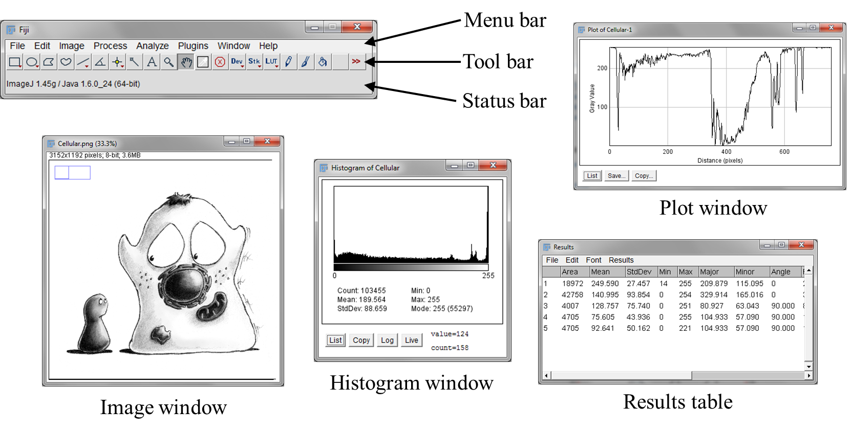
Figure 2: The main user interface for Fiji.
It can take some time to get used to the ImageJ/Fiji[3] user interface, which may initially seem less friendly and welcoming than that found in some commercial software. But the good news is that, once you find your way around, it becomes possible to do a lot of things that would simply not be possible in many other software applications.
Some of the components we will be working with are shown in Figure 2. At first, only the main window containing the menu, tool and status bars is visible, and the others appear as needed when images are opened and processed. Should you ever lose this main window behind a morass of different images, you can bring it back to the front by pressing the Enter key.
Tips & tricks
Here are a few non-obvious tips that can making working with ImageJ or Fiji easier, in order of importance (to me):
-
Files can be opened quickly by dragging them (e.g. from the desktop, Windows Explorer or the Mac Finder) onto the
Status bar. Most plugins you might download can also be installed this way. -
If you know the name of a command (including plugins) but forget where it is hidden amidst the menus, type Ctrl+L (or perhaps just L) to bring up the
Command Finder– it may help to think of it as a List – and start typing the name. You can run the command directly, or selectShow full informationto find out its containing menu. Note that some commands have similar or identical names, in which case they might only be distinguishable by their menu. -
ImageJ’s has very limited abilities – it may be available if you modify a single 2D image, but will not be if you process data with more dimensions (see Dimensions). While inconvenient if you are used to long undo-lists in software like Microsoft Word or Adobe Photoshop, there is a good rationale behind it: supporting undo could require storing multiple copies of previous versions of the image, which might rapidly use up all the available memory when using large data sets. The solution is to take care of this manually yourself by choosing to create a copy of the image before doing any processing you may not wish to keep.
-
There is a wide range of shortcut keys available. Although the menus claim you need to type Ctrl, you do not really unless the option under tells you otherwise. You can also add more shortcuts under
-
To move around large images, you can use the
scrolling tool , or
simply click and drag on the image while holding down the spacebar. A
small rectangular diagram (visible on the top left of the image window
in Figure 2) indicates which part of the entire image is
currently being shown.
, or
simply click and drag on the image while holding down the spacebar. A
small rectangular diagram (visible on the top left of the image window
in Figure 2) indicates which part of the entire image is
currently being shown. -
There are more tools and options than meet the eye. Double-clicking and right-clicking on icons in the
Tool barcan each reveal more possibilities. -
Pressing Escape may abort the operation of any currently-running command… But it requires the command’s author to have implemented this functionality. So it might not do anything.
Finding more information
Links to more information for using ImageJ, including user guides including a detailed manual, are available at http://imagej.net/Introduction.
Data & its display
Comparing images
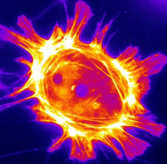
Now we return to the data/display dichotomy. In the top row of Figure 3, you can see four images as they might be shown in ImageJ. The first and second pairs both look identical to one another. However, it is only actually (A) and (C) that are identical in terms of content. Since these contain the original pixel values given by the microscope they could be analyzed, but analyzing either (B) or (D) instead may well lead to untrustworthy results.

|
|

|
|
A: 16-bit ('Grays' LUT)
|
B: 8-bit ('Grays' LUT)
|
C: 16-bit ('Fire' LUT)
|
D: 8-bit (RGB)
|
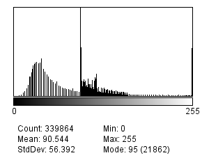
Figure 3: Do not trust your eyes for image comparisons: different pixel values might be displayed so that they look the same, while the same pixel values may be displayed so that they look different. Here, only the images in (A) and (C) are identical to one another in terms of their pixel values — and only these contain the original data given by the microscope. The terms used in the captions will be explained in Types & bit-depths and Channels & colors.
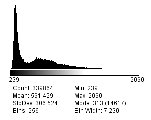
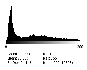
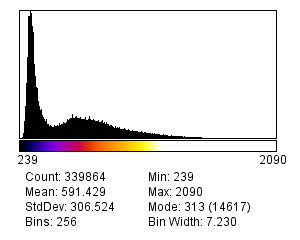
Reliably assessing the similarities and differences between images in Figure 3 would therefore be impossible just based on their appearance in the top row, but it becomes much easier if we consider the corresponding image histograms below. These histograms (created with ) depict the total number of pixels with each different value within the image as a series of vertical bars, displayed above some extra statistics – such as the maximum, minimum and mean of all the pixels in that image. Looking at the histograms and the statistics below make it clear that only (A) and (C) could possibly contain the same values.
Mapping colors to pixels
The reason for the different appearances of images in Figure 3 is that the first three do not all use the same lookup tables (LUTs; sometimes alternatively called color maps), while in (D) the image has been flattened. Flattening will become relevant in Channels & colors, but for now we will concentrate on LUTs.
A LUT is essentially a table in which rows give possible pixel values alongside the colors that should be used to display them. For each pixel in the image, ImageJ finds out the color of square to draw on screen by 'looking up' its value in the LUT. This means that when we want to modify how an image appears, we can simply change its LUT – keeping all our pixel values safely unchanged.
Practical
 Using
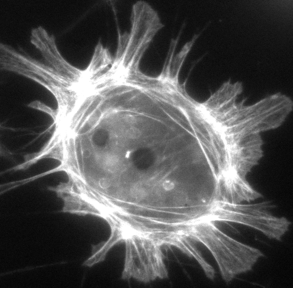
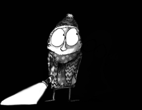
Using Spooked.tif as an example image, explore pixel values and LUTs
in Fiji. Originally, each pixel should appear with some shade of gray
(which indicates a correspondingly sombre LUT). As you move the cursor
over the image, in the status bar at the top of the screen you should
see value = beside the numerical value of whichever pixel is
underneath the cursor.
If you then go to and click on some other LUT the image appearance should be instantly updated, but putting the cursor over the same pixels as before will reveal that the actual values are unchanged.
Finally, if you want to 'see' the LUT you are using, choose
. This shows a bar stretching from 0 to 255 (the
significance of this range will be clearer after
reading Types & bit-depths) with the color given to each value in
between. Clicking List then shows the actual numbers involved in the
LUT, and columns for Red, Green and Blue. These latter columns
give instructions for the relative amounts of red, green and blue light
that should be mixed to get the right color (see
Channels & colors).
Why use different LUTs?
The ability to change LUTs has several advantages. A simple one is that
we can use LUTs to make the colors in our image match with the
wavelengths of the light we have detected, such as by showing a DAPI
staining in blue or GFP in green. But often this is not really optimal,
and you may prefer to show an image using some multicolored LUT (e.g.
Fire in ImageJ) that does not otherwise have any physical relevance.
This is because the eye is relatively poor at distinguishing different
shades of the same color, and presenting the identical information
using many different colors can make differences between pixel values
more apparent.
Modifying the LUT can help make information visible
But swapping one set of LUT colors for another is not the only way to change the appearance. We can also keep the same colors, but change which pixel values each color is used for.
For example, suppose we have chosen a gray LUT. Most monitors can (theoretically) show us 256 different shades of gray, so we can give a different shade to pixels with values from 0–255, where 0 corresponds to black and 255 corresponds to white. But suppose our image only contains interesting values in the range 5–50. Then we will only be using 46 rather similar shades of gray to display it, and not using either our monitor or our eyesight to their full capacities. It would easier to see what is happening if we made every pixel with a value ≤ 5 black and ≥ 50 white, and then distributed all our available shades of gray to the values in between. This would make full use of the colors we have in our LUT, and give us an image with improved contrast. Of course, we can also apply the same principle using any other LUT, replacing black and white with the first and last colors in the LUT respectively.
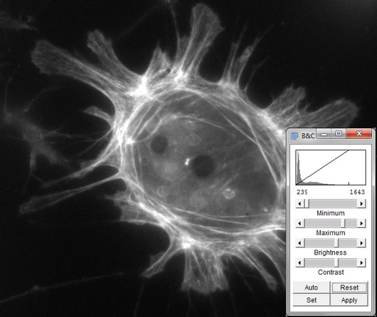
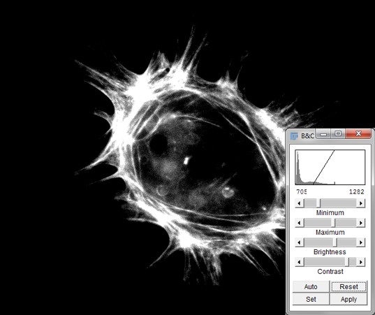
Adjusting the display range
A: Grayscale
|
B: Grayscale
|
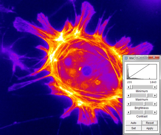
C: Fire LUT
|
Figure 4: The same image can be displayed in different ways by adjusting the contrast settings or the LUT. Nevertheless, despite the different appearance, the values of the pixels are the same in all three images.
This type of LUT adjustment is done in ImageJ using the
command (quickly accessed by
typing Shift+C; see Figure 4). The first two
scrollbars that appear are called Minimum and Maximum, and these
define the thresholds below and above which pixels are given the first
or last LUT color respectively. Modifying either of these sliders
automatically changes the Brightness and Contrast sliders.
Although the terms brightness and contrast are probably more familiar, it is
usually easier to work with Minimum and Maximum. If you know, for
example, you do not care to see anything in the darkest part of the
image, you can increase the value of Minimum to clip it out of the
picture (only for display!), and devote more different colors for the
part of the image that is really interesting.
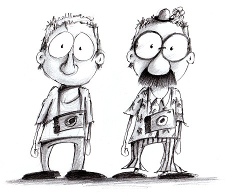
A: Fundamentally the same — despite different appearances
|
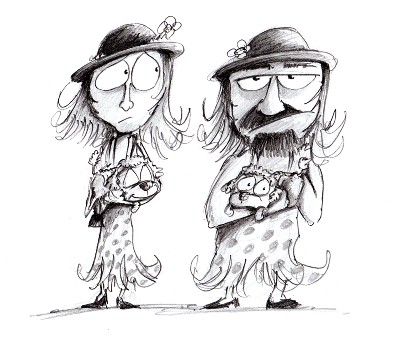
B: Fundamentally different — despite the same (or similar) appearance
|
Figure 5: The same person may appear very different thanks to changes in clothing and accessories (A). Conversely, quite different people might be dressed up to look very similar, and it is only upon closer inspection that significant differences become apparent (B). The true identity and dressing can be seen as analogous to an image’s pixel values and its display.
Properties & pixel size
Hopefully by now you are appropriately paranoid about accidentally changing pixel values and therefore compromising your image’s integrity, so that if in doubt you will always calculate histograms or other measurements before and after trying out something new to check whether the pixels have been changed.
This chapter ends with the other important characteristic of pixels for analysis: their size, and therefore how measuring or counting them might be related back to identifying the sizes and positions of things in real life. Sizes also need to be correct for much analysis to be meaningful.
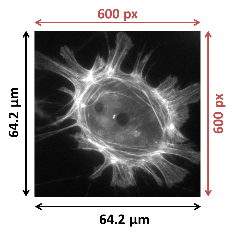
A: 600 × 600 pixel image and its properties
|

|
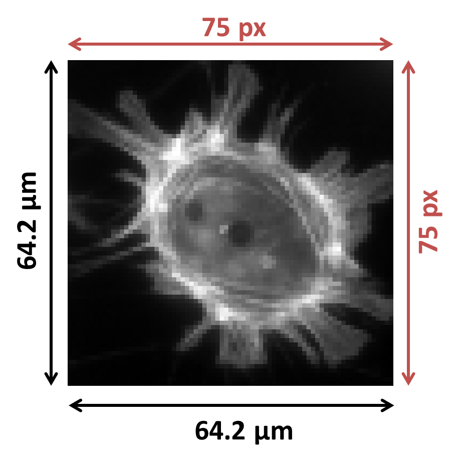
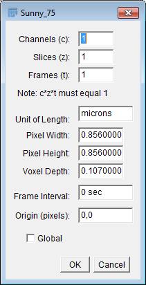
B: 75 × 75 pixel image and its properties
|
|
Figure 6: Two images with the same field of view, but different numbers of pixels — and therefore different pixel sizes. In (A) the pixel width and height are both 64.2µm / 600px = 0.107µm. In (B) the pixel width and height are both 64.2µm / 75px = 0.856µm/px. For display, (B) has been scaled up to look the same size as (A), so its larger pixels make it appear more 'blocky'.
Pixel sizes are found in ImageJ under , where you
will see values for Pixel width and Pixel height, defined in terms
of Unit of Length. A useful way to think of these is as proportions of
the size of the total field of view contained within the image (see
Figure 6). For example, suppose we are imaging an area with
a width of 100µm, and we have 200 pixels in the horizontal direction of
our image. Then we can treat the 'width' of a pixel as
100/200 = 0.5µm. The pixel height can be defined and used
similarly, and is typically (but not necessarily) the same as the width.
Pixel squareness
 Talking of pixels as having (usually) equal widths and
heights makes them sound very square-like, but earlier I stated that
pixels are not squares – they are just displayed using squares.
Talking of pixels as having (usually) equal widths and
heights makes them sound very square-like, but earlier I stated that
pixels are not squares – they are just displayed using squares.
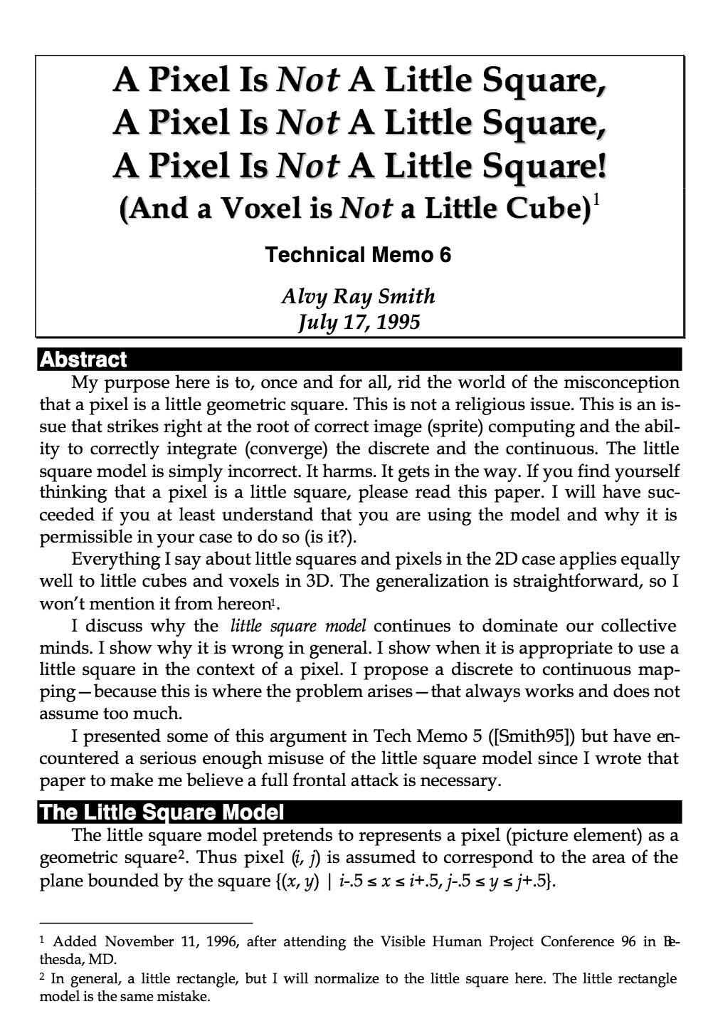
This slightly murky philosophical distinction is considered in Alvy Ray Smith’s technical memo (right), the title of which gives a good impression of the central thesis.[4] In short, pushing the pixels-are-square model too far leads to confusion in the end (e.g. what would happen at their 'edges'?), and does not really match up to the realities of how images are recorded (i.e. pixel values are not determined by detecting light emitted from little square regions, see Blur & the PSF). Alternative terms, such as sampling distance, are often used instead of pixel sizes – and are potentially less misleading. But ImageJ uses pixel size, so we will as well.
Pixel sizes and measurements
Knowing the pixel size makes it possible to calibrate size measurements. For example, if we measure some structure horizontally in the image and find that it is 10 pixels in length, with a pixel size of 0.5µm, we can deduce that its actual length in reality is (roughly!) 10 × 0.5µm = 5µm.
This calibration is often done automatically when things are measured in
ImageJ (see Measurements & regions of interest), and so the sizes must be correct for the
results to be reasonable. All being well, appropriate pixel sizes will be written into an
image file during acquisition and subsequently read – but this does not
always work out (see Files & file formats), and so Properties… should
always be checked. If ImageJ could not find sensible values in the image
file, by default it will say each pixel has a width and height of 1.0
pixel… not very informative, but at least not wrong. You can then
manually enter more appropriate values if you know them.
Pixel sizes and detail
In general, if the pixel size in a fluorescence image is large then we cannot see very fine detail (see Figure 6). However, the subject becomes complicated by the diffraction of light whenever we are considering scales of hundreds of nanometers, so that acquiring images with smaller pixel sizes does not necessarily bring us extra information – and might actually become a hindrance.
This will be explored in more detail in later chapters (Blur & the PSF and Noise).
1. All three of these consist of some computer-readable instructions, but they are written in slightly different languages. Macros are usually the easiest and fastest to write, and we will start producing our own in Writing macros. For more complex tasks, the others my be preferable.
2. The distinction between ImageJ and ImageJ2 does not need to concern us here, although if you are interested you can read more here. Also, if for any reason you would like to get ImageJ 'only', without the extras of ImageJ2 or Fiji, you still can at https://imagej.nih.gov/ij/
3. At the risk of confusion, I will refer to ImageJ most of the time, and Fiji only whenever discussing a feature not included within ImageJ.