-
Many processing operations can be extended into more than 2 dimensions
-
Adding extra dimensions can greatly increase the processing requirements
-
Objects can be detected & measured in 3D
Processing data with higher dimensions
Chapter outline
Introduction
So far, in terms of image processing we have concentrated only on 2D images. Most of the operations we have considered can also be applied to 3D data – and sometimes data with more dimensions, in cases where this is meaningful.
Point operations, contrast & conversion
Point operations are straightforward: they depend only on individual
pixels, so the number of dimensions is unimportant. Image arithmetic
involving a 3D stack and a 2D image can also be carried out in ImageJ
using the Image Calculator, where the operation involving the 2D image
is applied to each slice of the 3D stack in turn. Other options, such as
filtering and thresholding, are possible, but bring with them extra
considerations – and often significantly higher computational costs.
Setting the LUT of a 3D image requires particular care. The normal
Brightness/Contrast… tool only takes the currently-displayed slice
into consideration when pressing Reset or Auto. Optimizing the
display for a single slice does not necessarily mean the rest of the
stack will look reasonable if the brightness changes much.
is a better choice, since here you can
specify that the information in the entire stack should be used. You can
also specify the percentage of pixels that should be saturated (clipped)
for display, i.e. those that should be shown with the first or last
colors in the LUT. So long as Normalize and Equalize histogram are
not selected, the pixel values will not be changed.
3D filtering
Many filters naturally lend themselves to being applied to as many dimensions as are required. For example, a 3 × 3 mean filter can easily become a 3 × 3 × 3 filter if averaging across slices is allowed. Significantly, it then replaces each pixel by the average of 27 values, rather than 9. This implies the reduction in noise is similar to that of applying a 5 × 5 filter (25 values), but with a little less blurring in 2D and a little more along the third dimension instead. Several 3D filters are available under the submenu.
Fast, separable filters
The fact that 3D filters inherently involve more pixels is one reason that they tend to be slow. However, if a filter happens to have the very useful property of separability, then its speed can be greatly improved. Mean and Gaussian filters have this property, as do minimum and maximum filters (of certain shapes) – but not median.
The idea is that instead of applying a single n × n × n filter, three different 1D filters of length n can be applied instead – rotated so that they are directed along each dimension in turn. Therefore rather than n3 multiplications and additions being required to calculate each pixel in the linear case (e.g. see Filters), only 3n multiplications and additions are required. With millions of pixels involved, even when n is small the saving can be huge. Figure 1 shows the basic idea in 2D, but it can be extended to as many dimensions as needed. uses this approach.
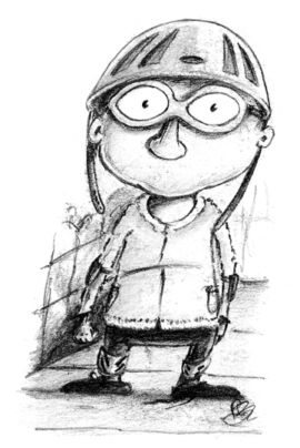
A: Original image
|
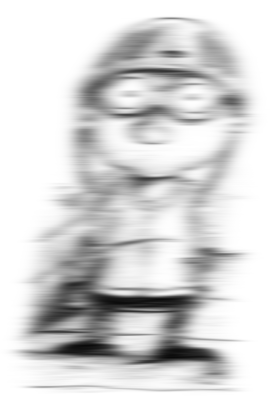
B: Horizontally smoothed (A)
|

C: Horizontally smoothed (B)
|
Figure 1: Smoothing applied separably using a 1D Gaussian filter (first aligned horizontally, then vertically) to an image or a rather well-protected young man seen playing safely on the streets of Heidelberg in 2010. The end result (C) is the same as what would be obtained by applying a single, 2D Gaussian filter to (A).
Dimensions & isotropy
If applying a filter in 3D instead of 2D, it may seem natural to define it as having the same size in the third dimension as in the original two. But for a z-stack, the spacing between slices is usually larger than the width and height of a pixel. And if the third dimension is time, then it uses another scale entirely. Therefore more thought usually needs to be given to what sizes make most sense.
In some commands (e.g. ), there is a
Use calibration option to determine whether the values you enter are
defined in terms of the units found in the Properties… and therefore
corrected for the stored pixel dimensions. Elsewhere (e.g.
Gaussian Blur 3D…) the units are pixels, slices and time points – and
so you are responsible for figuring out how to compensate for different
scales and units.
Thresholding multidimensional data
When thresholding an image with more than 2 dimensions using the
Threshold… command, it is necessary to choose whether the threshold
should be determined from the histogram of the entire stack, or from the
currently-visible 2D slice only. If the latter, you will also be asked
whether the same threshold should be used for every slice, or if it
should be calculated anew for each slice based upon the slice histogram.
In some circumstances, these choices can have a very large impact upon
the result.
Measurements in 3D data
ImageJ has good support for making measurements in 2D, particularly the
Measure and Analyze Particles… commands. The latter can happily
handle 3D images, but only by creating and measuring 2D ROIs
independently on each slice. Alternatively,
is like applying Measure to each
slice independently, making measurements either over the entire image or
any ROI. It will also plot the mean pixel values, but even if you do not
particularly want this the command can still be useful. However, if
single measurements should be made for individual objects that extend
across multiple slices, neither of these options would be enough.
Practical
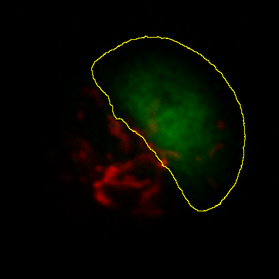
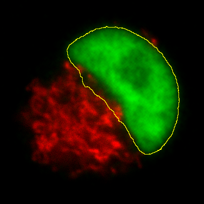
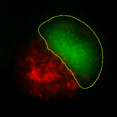
Suppose you have a cell, nucleus or some other large 3D structure in a z-stack,
and you want to draw the smallest 2D ROI that completely contains it on
every slice. An example is shown on the right for the green structure in
the Confocal Series sample image.
How would you create such a ROI, and be confident that it is large enough for all slices?
Answer
My strategy would be to create a z-projection (max intensity) and then draw the ROI
on this – or, preferably, create the ROI by thresholding using
and the Wand tool. This ROI can then be
transferred over to the original stack, either via the ROI Manager or
.
Practical
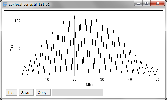
When I create a ROI on the sample image Confocal Series and run
Plot Z-axis Profile, I get a strangely spikey result (shown right).
How could this be explained?
(I used Fiji/ImageJ 1.46k. This behavior has been corrected since then.)
Answer
Confocal Series has two channels: it is a hyperstack (4D). But
Plot Z-axis Profile ignored this previously, and treated it like a
stack (3D). Therefore measurements from each channel were interleaved
with one another. Splitting the channels first, then calculating the
profiles separately would overcome this.
Histograms & threshold clipping
One way to measure in 3D is to use the Histogram command and specify
that the entire stack should be included – this provides some basic
statistics, including the total number, mean, minimum, maximum and
standard deviation of the pixels[2]. This will respect the
boundaries of a 2D ROI if one has been drawn.
This is a start, but it will not adjust to changes in the object
boundary on each 2D plane. A better approach could be to use
to set a threshold that identifies the
object – but do not press Apply to generate a binary image. Rather,
under select Limit to threshold. Then
when you compute the stack histogram (or press Measure for 2D) only
above-threshold pixels will be included in the statistics. Just be sure
to reset Limit to threshold later.
The 3D Objects Counter
Currently, the closest thing to Analyze Particles… for measuring
connected objects in 3D built-in to Fiji is the 3D Objects Counter
()[3]. Its settings (analogous
to Set Measurements…) are under . In addition
to various measurements, it provides labelled images as output, either
of the entire objects or only their central pixels – optionally with
labels, or expanded to be more visible.
2. Be careful! If you have multiple channels, these should be split first.
3. See See S Bolte and F P Cordelières. “A guided tour into subcellular colocalization analysis in light microscopy.” In: Journal of Microscopy 224.Pt 3 (Dec. 2006), pp. 213–32. url: http://www.ncbi.nlm.nih.gov/pubmed/17210054