-
Morphological operations can be used to refine or modify the shapes of objects in binary images
-
The distance & watershed transforms can be used to separate close, round structures
Binary images
Chapter outline
Introduction
By means of filtering and thresholding, we can create binary images to detect structures of various shapes and sizes for different applications. Nevertheless, despite our best efforts these binary images often still contain inaccurate or undesirable detected regions, and could benefit from some extra cleaning up. Since at this stage we have moved away from the pixel values of the original image and are working only with shapes – morphology – the useful techniques are often called morphological operations. In ImageJ, several of these are to be found in the submenu.
Morphological operations using rank filters
Erosion & dilation
Our first two morphological operations, erosion and dilation, are actually identical to minimum and maximum filtering respectively, described in the previous chapter. The names erosion and dilation are used more often when speaking of binary images, but the operations are the same irrespective of the kind of image. Erosion will make objects in the binary image smaller, because a pixel will be set to the background value if any other pixels in the neighborhood are background. This can split single objects into multiple ones. Conversely, dilation makes objects bigger, since the presence of a single foreground pixel anywhere in the neighborhood will result in a foreground output. This can also cause objects to merge.

A: Erosion
|

B: Dilation
|

C: Opening
|

D: Closing
|
Figure 1:
The effects of the Erode, Dilate, Open and Close-` commands.
The original image is shown at the top, while the processed part is at the bottom in each case.
Opening & closing
The fact that erosion and dilation alone affect sizes can be a problem: we may like their abilities to merge, separate or remove objects, but prefer that they had less impact upon areas and volumes. Combining both operations helps achieve this.
Opening consists of an erosion followed by a dilation. It therefore first shrinks objects, and then expands them again to an approximately similar size. Such a process is not as pointless as it may first sound. If erosion causes very small objects to completely disappear, clearly the dilation cannot make them reappear: they are gone for good. Barely-connected objects separated by erosion are also not reconnected by the dilation step.
Closing is the opposite of opening, i.e. a dilation followed by an erosion, and similarly changes the shapes of objects. The dilation can cause almost-connected objects to merge, and these often then remain merged after the erosion. If you wish to count objects, but these are wrongly subdivided in the segmentation, closing may therefore help make the counts more accurate.
These operations are implemented with the Erode, Dilate, Open and
Close- commands – but only using 3 × 3
neighborhoods. To perform the operations with larger neighborhoods,
you can simply use the Maximum… and Minimum… filters, combining
them to get opening and closing if necessary. Alternatively, in Fiji you
can explore .
Outlines, holes & maximum
Several more commands are to be found in the submenu.
The Outline command, predictably, removes all the interior pixels from
2D binary objects, leaving only the perimeters (Figure 2A).
Fill Holes would then fill these interior pixels in again, or indeed
fill in any background pixels that are completely surrounded by
foreground pixels (Figure 2B). Skeletonize shaves off
all the outer pixels of an object until only a connected central line
remains (Figure 2C). If you are analyzing linear
structures (e.g. blood vessels, neurons), then this command or those in
Fiji’s submenu may be helpful.

A: Outline
|

B: Fill holes
|

C: Skeletonize
|
Figure 2:
The effects of the Outline, Fill holes and Skeletonize commands.
Using image transforms
An image transform converts an image into some other form, in which the pixel values can have a (sometimes very) different interpretation. Several transforms are relevant to refining image segmentation.
The distance transform
The distance transform replaces each pixel of a binary image with the
distance to the closest background pixel. If the pixel itself is already
part of the background then this is zero (Figure 3C).
It can be applied using the command,
and the type of output given is determined by the EDM output option
under (where EDM stands for 'Euclidean
Distance Map'). This makes a difference, because the distance between
two diagonal pixels is considered
(by Pythagoras' theorem), so a 32-bit output can give more exact
straight-line distances without rounding.
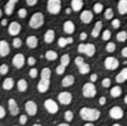
A: Original image
|

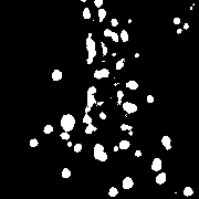
B: Thresholded image
|
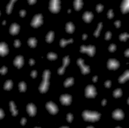
C: Distance transform
|
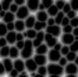
D: Distance transform of inverted thresholded image
|
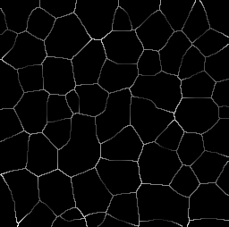
E: Voronoi
|
F: Voronoi + Ultimate points
|
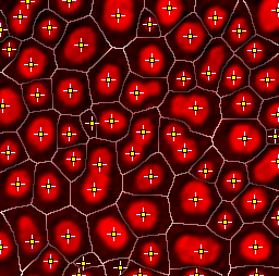
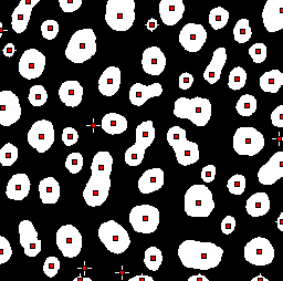
Figure 3:
Applying the distance transform and related commands to a segmented (using Otsu’s threshold) version of the sample image Blobs.
In (F), the original image is shown in the red channel, the Voronoi lines shown in gray and the ultimate points added as a Point selection.
A natural question when considering the distance transform is: why? Although you may not have a use for it directly, with a little creative thinking it turns out that the distance transform can help solve some other problems rather elegantly.
For example, Ultimate Points uses the distance transform to identify the
last points that would be removed if the objects would be eroded until
they disappear. In other words, it identifies centers. But these are not
simply single center points for each object; rather, they are maximum
points in the distance map, and therefore the pixels furthest away from
the boundary. This means that if a structure has several 'bulges', then
an ultimate point exists at the center of each of them. If segmentation
has resulted in structures being merged together, then each distinct
bulge could actually correspond to something interesting – and the
number of bulges actually means more than the number of separated
objects in the binary image (Figure 3F).
Alternatively, if the distance transform is applied to an inverted
binary image, the pixel values give the distance to the closest
foreground object (Figure 3D). With this, the
Voronoi command partitions an image into different regions so that the
separation lines have an equal distance to the nearest foreground
objects. Now suppose we detect objects in two separate channels of an
image, and we want to associate those in the second channel with the
closest objects in the first. We could potentially calculate the
distance of all the objects from one another, but this would be slow and
complicated. Simply applying Voronoi to the first channel gives us
different partitions, and then we only need to see which partition each
object in the second channel falls into (see Figure 3F).
This will automatically be the same partition as the nearest
first-channel object.
The watershed transform
The watershed transform provides an alternative to straightforward thresholding if you need to partition an image into many different objects. The idea behind it is illustrated in Figure 4.
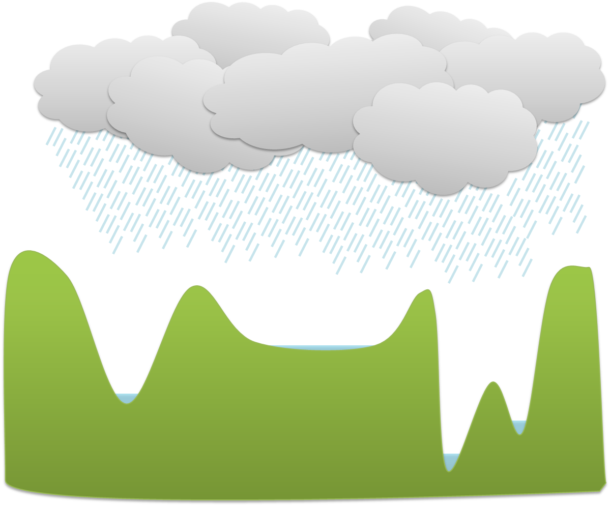
A: Water starts to fill the deepest regions first
|
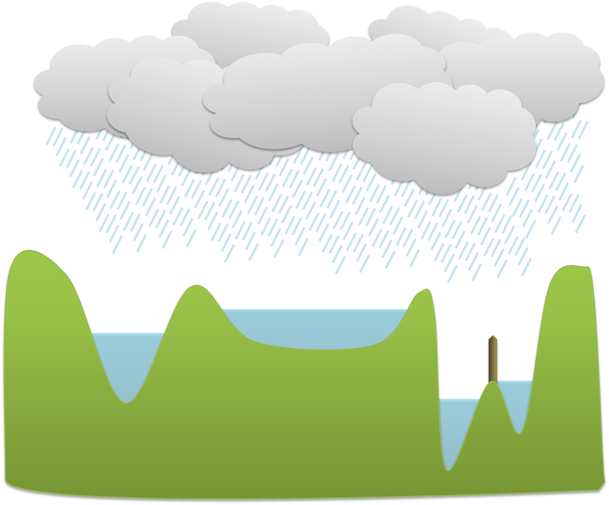
B: As the water rises, dams are built to prevent overflow
|
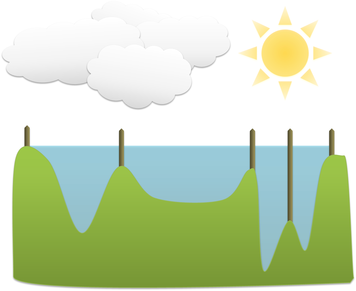
C: The water continues rising until reaching its maximum
|
Figure 4: A schematic diagram showing the operation of the watershed transform in 1 dimension. If you imagine rain falling on a hilly surface, the deepest regions fill up with water first. As the water rises further, soon the water from one of these regions would overflow into another region – in which case a dam is built to prevent this. The water continues to rise and dams added as necessary, until finally when viewed from above every location is either covered by water or belongs to a dam.
To understand how the watershed transform works, you should imagine the image as an uneven surface in which the value of each pixel corresponds to a height. Now imagine water falling evenly upon this surface and slowly flooding it. The water gathers first in the deepest parts; that is, in the places where pixels have values lower than all their neighbors. Each of these we can call a water basin.
As the water level rises across the image, occasionally it will reach a ridge between two basins – and in reality water could spill from one basin into the other. However, in the watershed transform this is not permitted; rather a dam is constructed at such ridges. The water then continues to rise, with dams being built as needed, until in the end every pixel is either part of a basin or a ridge, and there are exactly the same number of basins afterwards as there were at first.
ImageJ’s Watershed command is a further development of this general principle, in which the watershed
transform is applied to the distance transform of a binary image, where
the distance transform has also been inverted so that the centers of
objects (which, remember, are just the ultimate points mentioned
above) now become the deepest parts of the basins that will fill with
water. The end result is that any object that contains multiple ultimate
points has ridges built inside it, separating it into different objects.
If we happen to have wanted to detect roundish structures that were
unfortunately merged together in our binary image, then this may well be
enough to un-merge them (Figure 5).
A: Binary image + ultimate points
|

B: Watershed separation of objects in
|
C: Detail from thresholded image
|

D: Watershed separation of objects in (C)
|
Figure 5: Applying the watershed transform to binary images is able to separate some merged spots based upon their shape.