-
Point operations are mathematical operations applied to individual pixel values
-
They can be applied using a single image, an image and a constant, or two images of the same size
-
Some point operations improve image appearance by changing the relationships between pixel values
Manipulating individual pixels
Chapter outline
Introduction
A step used to process an image in some way is called an operation, and the simplest examples are point operations. These act on individual pixels, changing each in a way that depends upon its own value, but not upon where it is or the values of other pixels. While not immediately very glamorous, point operations often have indispensable roles in more interesting contexts – and so it is essential to know where to find them and how they are used.
Point operations using a single image
Arithmetic
The submenu is full of useful things to do with pixel
values. At the top of the list come the arithmetic operations: Add…,
Subtract…, Multiply… and Divide…. These might be used to
subtract background (extremely important when quantifying intensities;
see Simulating image formation) or scale the pixels of different
images into similar ranges (e.g. if the exposure time for one image was
twice that of the other, the pixel values should be divided by two to
make them more comparable) – and ought to mostly behave as you expect.
Image inversion
Inverting an image () effectively involves 'flipping' the intensities: making the higher values lower, and the lower values higher. In the case of 8-bit images, inverted pixel values can be easily computed simply by subtracting the original values from the maximum possible – i.e. from 255. Although this would work in principle for 16-bit images as well, it could have the slightly uncomfortable effect of making an image containing only small values suddenly now only contain huge ones.

A: Original image
|
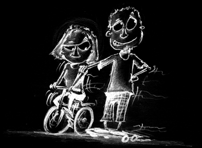
B: Inverted image
|
|
C: Inverted LUT
|
D: Inverted image + inverted LUT
|
Figure 1: The effect of image and LUT inversion on a depiction of two young lovers, spotted on Gaisbergstraße displaying the virtues of invention and tolerance.
Nonlinear contrast enhancement
With arithmetic operations we change the pixel values, usefully or
otherwise, but (assuming we have not fallen into the trap alluded to in
a previous question) we have done so in a linear way. At most it would
take another multiplication and/or addition to get us back to where we
were. Because a similar relationship between pixel values exists, we
could also adjust the Brightness/Contrast… so that it does not
look like we have done anything at all.
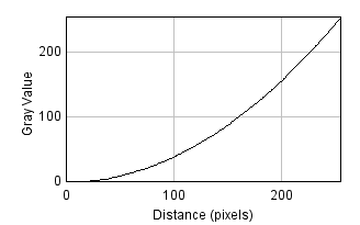
Nonlinear point operations differ in that they affect relative values
differently depending upon what they were in the first place
(Figure 2). This turns out to be very useful for
displaying images with high dynamic ranges – that is, a big difference
between the largest and smallest pixel values (e.g.
Figure 3). Using the Brightness/Contrast…
tool (which assigns LUT colors linearly to all the pixel values between
the minimum and maximum chosen) it might not be possible to find
settings that assign enough different colors to the brightest and
darkest regions simultaneously for all the interesting details to be
made visible.

|

|

|

|
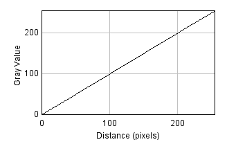
A: Original (linear)
|
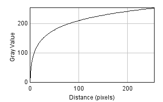
B: Log
|
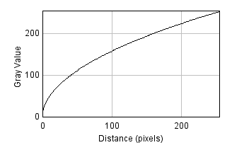
C: Gamma = 0.5
|
D: Gamma = 2.0
|
Figure 2: Nonlinear transforms applied to a simple 'ramp' image, consisting of linearly increasing pixel values. Replacing each pixel with its log or gamma-adjusted value has the effect of compressing either the lower or higher intensities closer together to free up more gray levels for the others.
The Gamma… or Log… commands within the submenu
offer one type of solution. The former means that every pixel with a
value p is replaced by pγ, where
γ is some constant of your choosing. The latter
simply replaces pixel values with their natural logarithm. Examples of
these are shown in Figure 3. Some extra (linear)
rescaling is applied internally by ImageJ when using gamma and log
commands, since otherwise the resulting values might fall out of the
range supported by the bit-depth.
A: Original image
|
B: Linear contrast
|
C: Gamma adjusted
|
D: Log transform
|
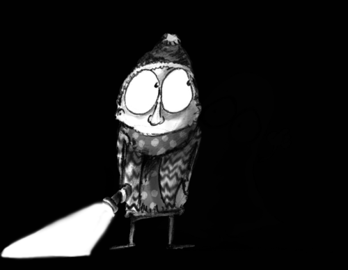
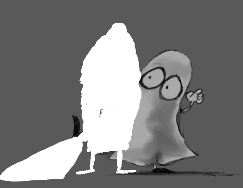
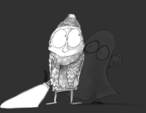
Figure 3: The application of nonlinear contrast enhancement to an image with a wide range of values. (Top row) In the original image, it is not possible to see details in both the foreground and background simultaneously. (Bottom row) Several examples of nonlinear techniques that make details visible throughout the image.
Point operations involving multiple images
Instead of applying arithmetic using an image and a constant, we could also use two images of the same size. These can readily be added, subtracted, multiplied or divided by applying the operations to the corresponding pixels.
The command to do this is found under . But
beware of the bit-depth! If any of the original images are 8 or 16-bit,
then the result might require clipping or rounding, in which case
selecting the option to create a 32-bit (float) result may be
necessary to get the expected output.
Question
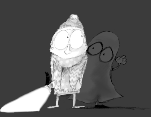
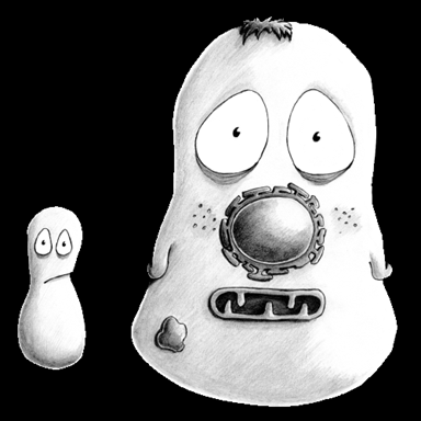
In the two 32-bit images shown here, white pixels have values of one and black pixels have values of zero (gray pixels have values somewhere in between).
|
|
What would be the result of multiplying the images together? And what would be the result of dividing the left image by the right image?
Answer
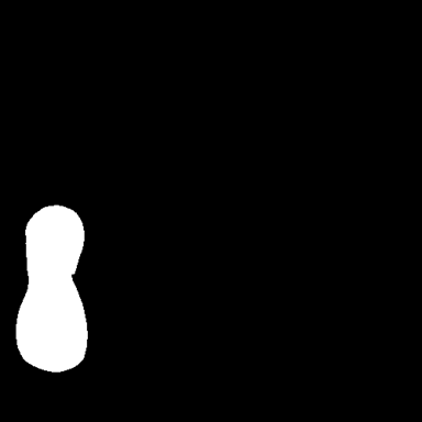
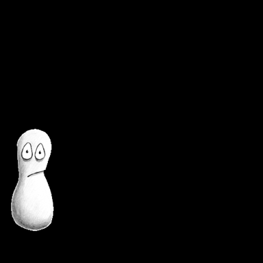
Multiplying the images effectively results in everything outside the white region in the right image being removed from the left image (i.e. set to zero).
|
Dividing has a similar effect, except that instead of becoming zero the masked-out pixels will take one of three results, depending upon the original pixel’s value in the left image:
-
if it was positive, the result is
-
if it was negative, the result is
-
if it was zero, the result is
NaN('not a number' – indicating 0/0 is undefined)
These are special values that can be contained in floating point images, but not images with integer types.
Modelling image formation: Adding noise
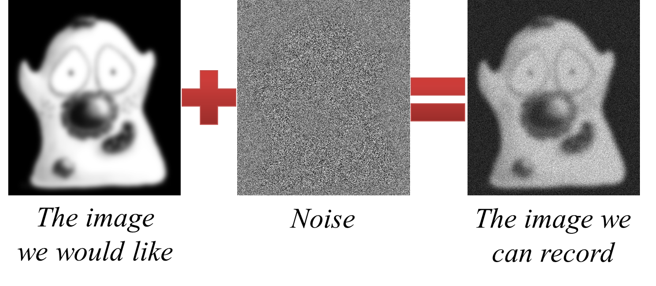
Fluorescence images are invariably noisy. The noise appears as a graininess throughout the image, which can be seen as arising from a random noise value (positive or negative) being added to every pixel. This is equivalent to adding a separate 'noise image' to the non-existent cleaner image that we would prefer to have recorded. If we knew the pixels in the noise image then we could simply subtract it to get the clean result – but, in practice, their randomness means that we do not.
|
Nevertheless, even the idea of a noise image being added is extremely useful. We can use it to create simulations in which the noise behaves statistically just like real noise, and add it to clean images. Using these simulations we can figure out things like how processing steps or changes during acquisition will affect or reduce the noise, or how sensitive our measurement strategies are to changes in image quality (see Filters, Noise and Simulating image formation).