-
The process of detecting interesting objects in an image is called segmentation, and the result is often a binary or labeled image
-
Global thresholding identifies pixels with values in particular ranges
-
Thresholds can be calculated from image histograms
-
Combining thresholding with filtering & image subtraction make it suitable for a wide range of images
-
Binary images can be used to create ROIs or other object representations
Detection by thresholding
Chapter outline
Introduction
Measurements & regions of interest described how measurements can be made using manually-drawn ROIs. This may be fine in simple cases where there are not too many things to analyze, but it is preferable to find ways to automate the process of defining regions – not only because this is likely to be faster, but because it should give more reproducible and less biased results.
Objects, segmentation, binary & labeled images
In image processing literature, interesting image structures are frequently called objects (or sometimes connected components), and the often troublesome process of detecting them is image segmentation.
Most of the techniques described in the following chapters can be strung together in an effort to segment an image accurately. If successful, the result may be a binary image, in which each pixel can only have one of two values to indicate whether it is part of an object or not, or a labeled image, in which all pixels that are part of the same object have the same, unique value. It is common to concentrate first on producing a binary image, and then create a labeled image only if necessary by identifying distinct clusters of object pixels and assigning the labels to these.
Global thresholding
The usual way to generate a binary image is by thresholding: identifying pixels above or below a particular threshold value. In ImageJ, the command allows you to define both low and high threshold values, so that only pixels falling within a specified range are found. After choosing suitable thresholds, pressing Apply produces the binary image[1]. Because the same thresholds are applied to every pixel in the entire image, this is an example of global thresholding – which is really a kind of point operation, since the output for any pixel depends only on the pixel’s original value and nothing else.
Choosing your results with manual thresholds
The puzzle of global thresholding is how to define the thresholds
sensibly. If you open and split the
channels (), you can use Threshold…
to interactively try out different possibilities for each channel. You
should soon notice the danger in this: the results (especially in the
red or green channels) can be very sensitive to the threshold you
choose. Low thresholds tend to detect more structures, and also to
make them bigger – until the point at which the structures merge, and
then there are fewer detected again
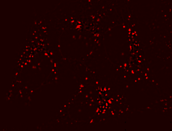
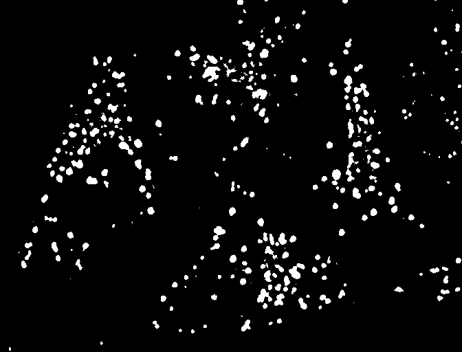
(Figure 1).
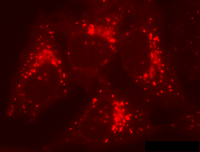
A: Image
|
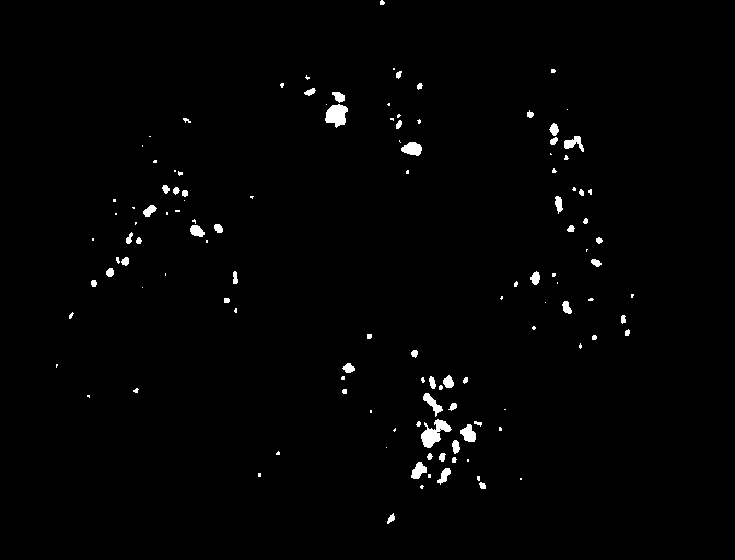
B: Low threshold
|
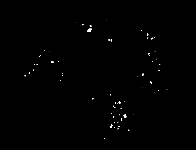
C: High threshold
|
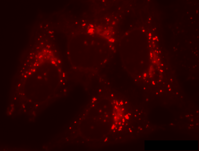
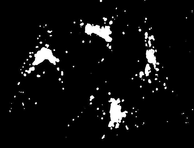
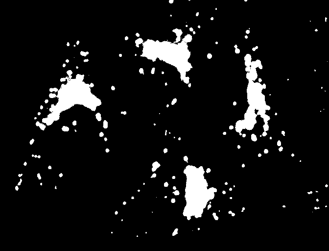
Figure 1:
Applying manually-chosen thresholds to the red channel of HeLa Cells (A).
In (B), a relatively low threshold results in 124 spots being detected with an average area of 32.9 pixels2 – but in some places these look like several spots merged.
Choosing a higher threshold to avoid merging leads to 74 detections in (C), with an average size of 20.3 pixels2.
In other words, you can sometimes use manual thresholds to get more or
less whatever result you want – which could completely alter the
interpretation of the data. For the upstanding scientist who finds this
situation disconcerting, ImageJ therefore offers a number of automated
threshold determination methods in a drop-down list in the
Threshold… tool. These are described at
http://imagej.net/Auto_Threshold, often with references to
the original published papers upon which they are based. Fiji’s
command provides additional options,
including the ability to apply all the thresholds and see which one
appears to provide the best results.
Determining thresholds from histograms
There is no always-applicable strategy to determine a threshold; images vary too much. However, by its nature, thresholding assumes that there are two classes of pixel in the image – those that belong to interesting objects, and those that do not – and pixels in each class have different intensity values[2]. Whenever values are significant, but their exact location in the image is either unknown or unimportant, this information is neatly summarized within the image’s histogram. Therefore ImageJ’s methods to find thresholds do not work on the images directly, but rather on their histograms – which is considerably simpler.
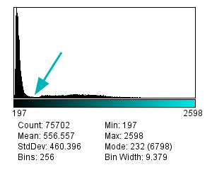
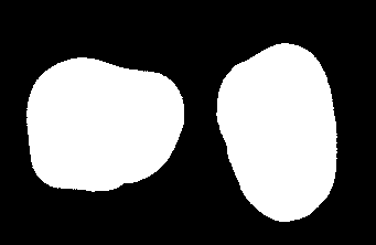
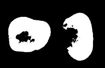
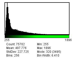
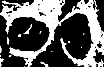
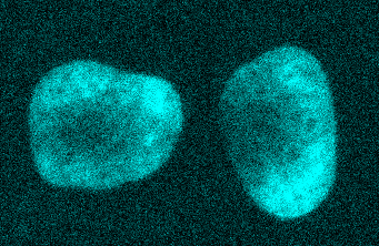
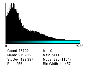
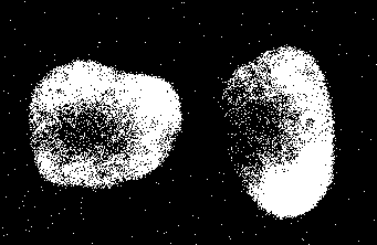
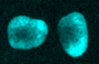
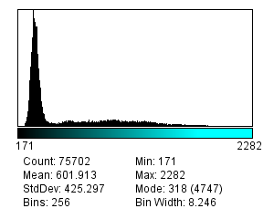
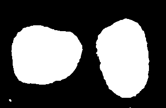
A justification for this can be seen in Figure 2. Looking at the image, the two nuclei are obvious: they clearly have higher values than the background (A). However, looking at the histogram alone (B) we could already have inferred that there was a class of background pixels (the tall peak on the left) and a class of 'other', clearly distinct pixels (the much shallower peak on the right). By choosing a threshold between these two peaks – somewhere around 400 – the nuclei can be cleanly separated (C). Choosing a threshold much higher or lower than this yields less impressive results (D).
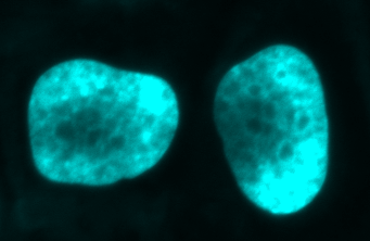
A: Image
|
B: Histogram
|
C: Triangle threshold
|
D: Otsu’s threshold
|
Figure 2:
Automated thresholding to detect nuclei.
(A) Detail from the blue channel of HeLa Cells.
(B) In the image histogram you can see one large peak corresponding to the background, and a much longer, shallower peak corresponding to the nuclei.
The arrow marks the trough between these two peaks.
From inspecting the histogram, one would expect that a threshold anywhere in the range 380-480 could adequately separate the two classes.
The triangle method yields a suitable threshold of 395 (C), while Otsu’s method gives 762, making it inappropriate for this particular data (D).
Figure 3 gives a more challenging example. In the image itself the structures are not very clearly defined, and in many cases it is not obvious whether we would want to consider any particular pixel as 'bright enough' for detection or not (A). The histogram also depicts this uncertainty; there is a smoother transition between the background peak and the foreground (B). The results of applying two different automated thresholds are shown, (C) and (D). Both are in some sense justifiable, and deciding which is the most appropriate would require a deeper understanding of what the image contains and what is to be analyzed.
A: Image
|
B: Histogram
|
C: Triangle threshold
|

D: Otsu’s threshold
|
Figure 3: Automated thresholding of less distinct classes. (A) Detail from the green channel of HeLa Cells. (B) The background peak is still visible in the histogram, but merges without an obvious trough into the foreground. The triangle method here gives a much lower threshold than Otsu’s method (461 rather than 615), although which is preferable may depend on the application (C)-(D).
Thresholding difficult data
Applying global thresholds is all well and good in easy images for which a threshold clearly exists, but in practice things are rarely so straightforward – and often no threshold, manual or automatic, produces useable results. This section anticipates the next chapter on filters by showing that, with some extra processing, thresholding can be redeemed even if it initially seems to perform badly.
Thresholding noisy data
Noise is one problem that affects thresholds, especially in live cell imaging. The top half of Figure 4 reproduces the nuclei from Figure 2, but with extra noise added to simulate less than ideal imaging conditions. Although the nuclei are still clearly visible in the image (A), the two classes of pixel previously easy to separate in the histogram have now merged together (B). The triangle threshold method, which had performed well before, now gives less attractive results (C), because the noise has caused the ranges of background and nuclei pixels to overlap. However, applying a Gaussian filter smooths the image, thereby reducing much of the random noise (see Filters), which results in a histogram dramatically more similar to that in the original, (almost) noise-free image, and the threshold is again quite successful (F).
A: Noisy image
|
B: Histogram of (A)
|
C: Threshold applied to (A)
|
D: Gaussian filtered image
|
E: Histogram of (D)
|
F: Threshold applied to (D)
|
Figure 4: Noise can affect thresholding. After the addition of simulated noise to the image in Figure 2, the distinction between nuclei and non-nuclei pixels is much harder to identify in the histogram (B). Any threshold would result in a large number of incorrectly-identified pixels. However, applying a Gaussian filter (here, sigma = 2) to reduce noise can dramatically improve the situation (E). Thresholds in (C) and (F) were computed using the triangle method.
Local thresholding
Another common problem is that structures that should be detected appear
on top of a background that itself varies in brightness. For example, in
the red channel of HeLa cells there is no single global threshold
capable of identifying and separating all the 'spot-like' structures;
any choice will miss many of the spots because a threshold high enough
to avoid the background will also be too high to catch all the spots
occurring in the darker regions (Figure 5a–c).
A: Original image
|
B: Otsu’s threshold
|
C: Triangle threshold
|
D: Median filtered image
|
E: Result of (A)-(D)
|
F: Triangle threshold of (E)
|
Figure 5: Thresholding to detect structures appearing on a varying background. No global threshold may be sufficiently selective (top row). However, if a 'background image' can be created, e.g. by median filtering, and then subtracted, a single threshold can give better results (bottom row). This is equivalent to applying a varying threshold to the original image.
In such cases it would be better if we could define different thresholds for different parts of the image: a local threshold. A few methods to do this are implemented in Fiji’s , and described at http://imagej.net/Auto_Local_Threshold. However, if these are insufficient it is easy to implement our own local thresholding and get more control over the result if we think of the problem from a slightly different angle. Suppose we had a second image that contained values equal to the thresholds want to apply, and which could be different for every pixel. If we simply subtract this second image from the first, we can then apply a global threshold to detect what we want.
The difficult part is creating the second image, but again filters come in useful. One option is a median filter, which effectively moves through every pixel in the image, ranks the nearby pixels in order of value, and chooses the middle one – thereby removing anything much brighter or much darker than its surroundings (D). Subtracting the median-filtered image from the original gives a result to which a global threshold can be usefully applied (E).
Practicalities: bit-depths & types
Using NaNs
Although not obviously integral to the idea of thresholding, bit-depths and image types are relevant in two main ways.
The first appears when
you click Apply in the Threshold… dialog box for a 32-bit image.
This presents the option Set Background Pixels to NaN, which instead
of making a binary image would give give an image in which the
foreground pixels retain their original values, while background pixels
are Not A Number. This is a special value that can only be stored in
floating point images, which ImageJ ignores when making measurements
later. It is therefore used to mask out regions.
Histogram binning
The second way in which bit-depths and types matter is that histograms of images > 8-bit involve binning the data. For example, with a 32-bit image it would probably not make sense to create a histogram that has separate counts for all possible pixel values: in addition to counts for pixels with exact values 1 and 2, we would have thousands of counts for pixels with fractions in between (and most of these counts would be 0). Instead, the histogram is generated by dividing the total data range (maximum – minimum pixel values) into 256 separate bins with equal widths, and counting how many pixels have values falling into the range of each bin. It is therefore like a subtle conversion to 8-bit precision for the threshold calculation, but without actually changing the original data. The same type of conversion is used for 16-bit images – unless you use Fiji’s command, which uses a full 16-bit histogram with 65536 bins.
Although binning effects can often be ignored, if the total range of pixel values in an image is very large then it is worth keeping in mind.
Measuring objects in binary images
Generating & measuring ROIs
Once we have a binary image, the next step is to identify objects within it and measure them. In 2D, there are several options:
-
Click on an object with the
Wandtool to create measurable ROI from it -
makes a single ROI containing all the foreground pixels. Disconnected regions can be separated by adding the ROI to the ROI Manager and choosing
More >> Split. -
detects and measures all the foreground regions as individual objects.
Analyze Particles… is the most automated and versatile option,
making it possible to ignore regions that are particularly small or
large, straight or round (using a Circularity metric). It can also
output summary results and add ROIs for each region to the ROI Manager.
With the Show: Count Masks option, it will generate a labeled image,
in which each pixel has a unique integer value indicating the number of
the object it is part of – or zero if it is in the background. With a
suitably colorful LUT, this can create a helpful and cheerful display
(Figure 6).
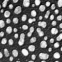
A: Original blobs
|

B: Binary image
|
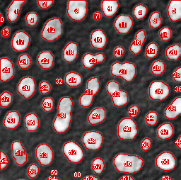
C: Original + ROIs
|

D: Labelled image
|
Figure 6:
Examples of a grayscale (Blobs.gif), binary and labelled image.
In (C), ROIs have been generated from (B) and superimposed on top of (A).
In (D), each label has been assigned a unique color for display.
Connectivity
Identifying multiple objects in a binary image involves separating distinct groups of pixels that are considered 'connected' to one another, and then creating a ROI or label for each group. Connectivity in this sense can be defined in different ways. For example, if two pixels have the same value and are immediately beside one another (above, below, to the left or right, or diagonally adjacent) then they are said to be 8-connected, because there are 8 different neighboring locations involved. Pixels are 4-connected if they are horizontally or vertically adjacent, but not only diagonally.
4-connected
|

8-connected
|
The choice of connectivity can make a big difference in the number and
sizes of objects found, as the example on the right shows (distinct
objects are shown in different colors). An option to specify the
connectivity used by the Wand tool can be found by double-clicking its
button.
Redirecting measurements
Although binary images can show the shapes of things to be measured,
pixel intensity measurements made on a binary image are not very
helpful. You could use the above techniques to make ROIs from binary
images, then apply those to the original image to get meaningful
measurements. However, it is possible to avoid this extra step by
changing the Redirect to: option under Set Measurements…. This
allows you to measure ROIs or run Analyze Particles… with one image
selected and used to define the regions, while redirecting your
measurements to be made on a completely different image of your choice.
If you use this, just be sure to reset the Redirect to: option when
you are done, to avoid accidentally measuring the wrong image for so
long as it is open.
1. Since in ImageJ this replaces the original image, you might want to duplicate it first.
2. Of course there may be multiple classes for different kinds of objects, and perhaps multiple thresholds would make more sense. However, in such cases it may be possible to apply steps such as filtering to remove some of the more confusing information, and reduce the detection problem to that of separating only two classes. Therefore although thresholding is not always appropriate and different methods of detection can be needed for complex problems, it is still useful a lot of the time.