Noise

Chapter outline

There are two main types of noise in fluorescence microscopy: photon noise & read noise
Photon noise is signal-dependent, varying throughout an image
Read noise is signal-independent, and depends upon the detector
Detecting more photons reduces the impact of both noise types

Introduction

We could reasonably expect that a noise-free microscopy image should look pleasantly smooth, not least because the convolution with the PSF has a blurring effect that softens any sharp transitions. Yet in practice raw fluorescence microscopy images are not smooth. They are always, to a greater or lesser extent, corrupted by noise. This appears as a random 'graininess' throughout the image, which is often so strong as to obscure details.

This chapter considers the nature of the noisiness, where it comes from, and what can be done about it. Before starting, it may be helpful to know the one major lesson of this chapter for the working microscopist is simply:

If you want to reduce noise, you need to detect more photons

This general guidance applies in the overwhelming majority of cases when a good quality microscope is functioning properly. Nevertheless, it may be helpful to know a bit more detail about why – and what you might do if detecting more photons is not feasible.

Background

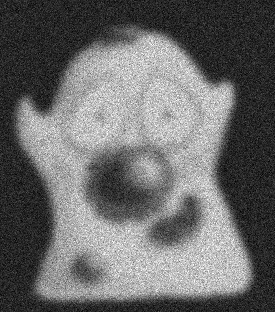
A: Noisy image

B: Ideal image

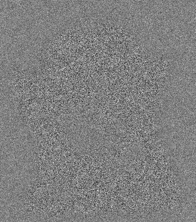
C: Result of (A) - (B)

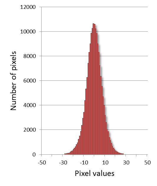
D: Histogram of (A) - (B)

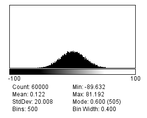
Figure 1: Illustration of the difference between a noisy image that we can record (A), and the noise-free (but still blurred) image we would prefer (B). The 'noise' itself is what would be left over if we subtracted one from the other (C). The histogram in (D) resembles a normal (i.e. Gaussian) distribution and shows that the noise consists of positive and negative values, with a mean of 0.

In general, we can assume that noise in fluorescence microscopy images has the following three characteristics, illustrated in Figure 1:

Noise is random – For any pixel, the noise is a random positive or negative number added to the 'true value' the pixel should have.
Noise is independent at each pixel – The value of the noise at any pixel does not depend upon where the pixel is, or what the noise is at any other pixel.
Noise follows a particular distribution – Each noise value can be seen as a random variable drawn from a particular distribution. If we have enough noise values, their histogram would resemble a plot of the distribution^[1].

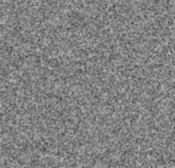
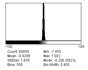
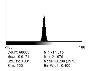
There are many different possible noise distributions, but we only need to consider the Poisson and Gaussian cases. No matter which of these we have, the most interesting distribution parameter for us is the standard deviation. Assuming everything else stays the same, if the standard deviation of the noise is higher then the image looks worse (Figure 2).

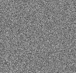
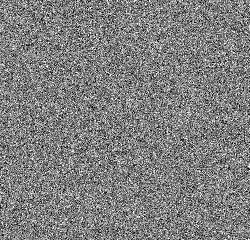
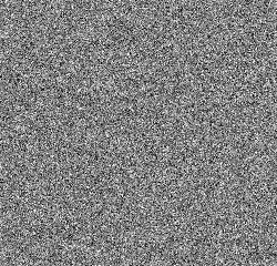
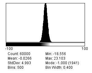
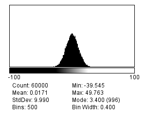
A: Std. dev. 5

B: Std. dev. 10

C: Std. dev. 20

Figure 2: Gaussian noise with different standard deviations. (Top) Noise values only, shown as images (with contrast adjusted) and histograms. (Bottom) Noise values added to an otherwise noise-free image, along with the resulting histograms. Noise with a higher standard deviation has a worse effect when added to an image.

The reason we will consider two distributions is that there are two main types of noise for us to worry about:

Photon noise, from the emission (and detection) of the light itself. This follows a Poisson distribution, for which the standard deviation changes with the local image brightness.
Read noise, arising from inaccuracies in quantifying numbers of detected photons. This follows a Gaussian distribution, for which the standard deviation stays the same throughout the image.

Therefore the noise in the image is really the result of adding two^[2] separate random components together. In other words, to get the value of any pixel $P$ you need to calculate the sum of the 'true' (noise-free) value $T$ , a random photon noise value $N_p$ , and a random read noise value $N_r$ , i.e.

$P = T + N_p + N_r$

Finally, some useful maths: suppose we add two random noisy values together. Both are independent and drawn from distributions (Gaussian or Poisson) with standard deviations $\sigma_1$ and $\sigma_2$ . The result is a third random value, drawn from a distribution with a standard deviation $\sqrt{\sigma_1 + \sigma_2}$ . On the other hand, if we multiply a noisy value from a distribution with a standard deviation $\sigma_1$ by $k$ , the result is noise from a distribution with a standard deviation $k\sigma_1$ .

These are all my most important noise facts, upon which the rest of this chapter is built. We will begin with Gaussian noise because it is easier to work with, found in many applications, and widely studied in the image processing literature. However, in most fluorescence images photon noise is the more important factor.

Gaussian noise

Gaussian noise is a common problem in fluorescence images acquired using a CCD camera (see Microscopes & detectors). It arises at the stage of quantifying the number of photons detected for each pixel. Quantifying photons is hard to do with complete precision, and the result is likely to be wrong by at least a few photons. This error is the read noise.

Read noise typically follows a Gaussian distribution and has a mean of zero: this implies there is an equal likelihood of over or underestimating the number of photons. Furthermore, according to the properties of Gaussian distributions, we should expect around ~68% of measurements to be ±1 standard deviation from the true, read-noise-free value. If a detector has a low read noise standard deviation, this is then a good thing: it means the error should be small.

Signal-to-Noise Ratio (SNR)

Read noise is said to be signal independent: its standard deviation is constant, and does not depend upon how many photons are being quantified. However, the extent to which read noise is a problem probably does depend upon the number of photons. For example, if we have detected 20 photons, a noise standard deviation of 10 photons is huge; if we have detected 10 000 photons, it is likely not so important.

A better way to assess the noisiness of an image is then the ratio of the interesting part of each pixel (called the signal, which is here what we would ideally detect in terms of photons) to the noise standard deviation, which together is known as the Signal-to-Noise Ratio^[3]:

$\textrm{SNR} = \frac{\textrm{Signal}}{\textrm{Noise standard deviation}}$

Question

Calculate the SNR in the following cases:

We detect an average of 10 photons, read noise standard deviation 1 photon
We detect an average of 100 photons, read noise standard deviation 10 photons
We detect an average of 1000 photons, read noise standard deviation 10 photons

For the purposes of this question, you should assume that read noise is the only noise present (ignore photon noise).

Answer

We detect an average of 10 photons, read noise std. dev. 1 photon: SNR = 10
We detect an average of 100 photons, read noise std. dev. 10 photons: SNR = 10
We detect an average of 1000 photons, read noise std. dev. 10 photons: SNR = 100

The noise causes us a similar degree of uncertainty in the first two cases. In the third case, the noise is likely to be less problematic: higher SNRs are good.

Gaussian noise simulations

I find the best way to learn about noise is by creating simulation images, and exploring their properties through making and testing predictions. Process ▸ Noise ▸ Add Specified Noise… will add Gaussian noise with a standard deviation of your choosing to any image. If you apply this to an empty 32-bit image created using File ▸ New ▸ Image… you can see noise on its own.

Practical

Create an image containing only simulated Gaussian noise with a standard deviation of approximately 3. Confirm using its histogram or the Measure command that this standard deviation is correct.

Now add to this more Gaussian noise with a standard deviation of 4. Keeping in mind the end of the background section, what do you expect the standard deviation of the result to be?

Answer

The standard deviation of the result should be close to $\sqrt{9 + 16} = 5$

Question

gauss_noise_1.tif and gauss_noise_2.tif are two images containing Gaussian noise with standard deviations of 5. Estimate (and optionally test with Image Calculator… and Measure), what the standard deviations will be:

When you add both images together
When you subtract gauss_noise_2.tif from gauss_noise_1.tif
When you subtract gauss_noise_1.tif from gauss_noise_2.tif
When you average both images together
When you add an image to itself

Answer

When operating on the noise images with standard deviations of 5, the (approximate) standard deviations you should get are:

$\sqrt{50} = 7.1$ – add the variances, then take the square root
$\sqrt{50} = 7.1$ – same as addition; switching the sign (positive or negative) of a Gaussian noise image with zero mean just gives another Gaussian noise image with zero mean
$\sqrt{50} = 7.1$ – the order of subtraction doesn’t matter
$\sqrt{50}/2 = 3.5$ – same as addition, but divide the result by 2
$10$ – equivalent to multiplying the image by 2, so multiply the standard deviation by 2

Averaging noise

At the beginning of this chapter it was stated how to calculate the new standard deviation if noisy pixels are added together (i.e. it is the square root of the sum of the original variances). If the original standard deviations are the same, the result is always something higher. But if the pixels are averaged, then the resulting noise standard deviation is lower.

This implies that if we were to average two independent noisy images of the same scene with similar SNRs, we would get a result that contains less noise, i.e. a higher SNR. This is the idea underlying our use of linear filters to reduce noise in Filters, except that rather than using two images we computed our averages by taking other pixels from within the same image (Figures 4).

A: Original image

B: Averaging 2 adjacent pixels

C: Averaging 9 adjacent pixels

Figure 3: Noise reduction by averaging adjacent pixels.

A: Std. dev. 5

B: Std. dev. 10

C: Std. dev. 20

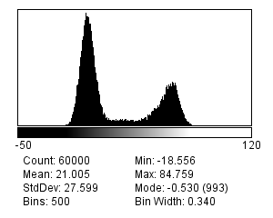
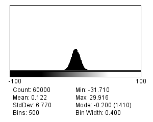
Figure 4: Images and histograms from Figure 2 after replacing each pixel with the mean of it and its immediate neighbors (a 3 × 3 mean filter). The standard deviation of the noise has decreased in all cases. In the noisiest example (C) the final image may not look brilliant, but the peaks in its histogram are clearly more separated when compared to Figure 2C, suggesting it could be thresholded more effectively. It is not always the most aesthetically pleasing image that is the best for analysis.

Practical

Create another image containing simulated Gaussian noise with a standard deviation of 30. What do you expect the standard deviation to be after applying a 3 × 3 mean filter (e.g. Process ▸ Smooth)? The calculation you need is much the same as in the last practical, but with some extra scaling involved.

Now apply the filter to the same image a second time. Is the noise reduced by a similar amount? How do you explain your answer?

Answer

After applying the filter once, the standard deviation should be around 10. Using a 3 × 3 mean filter, the noise standard deviation should be reduced to around 1/3 of its original value.

You can break down the problem this way:

Let the original noise standard deviation be $\sigma$ , the variance is $\sigma^2$
The filter first replaces each pixel with the sum of 9 independent values. The variance becomes $9\sigma^2$ , the standard deviation $\sqrt{9\sigma^2} = 3\sigma$
The filter divides the result by 9 to give means. This also divides the standard deviation by 9, giving $3\sigma/9 = \sigma/3$

However, when I apply the filter a second time, the standard deviation is 7. It has decreased by much less, despite using the same filter. This is because after the first filtering, the noise is no longer independent at each pixel.

Poisson noise

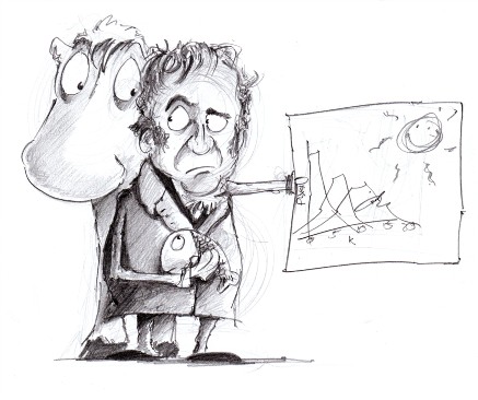
In 1898, Ladislaus Bortkiewicz published a book entitled The Law of Small Numbers. Among other things, it included a now-famous analysis of the number of soldiers in different corps of the Prussian cavalry who were killed by being kicked by a horse, measured over a 20-year period. Specifically, he showed that these numbers follows a Poisson distribution.

This distribution, introduced by Siméon Denis Poisson in 1838, gives the probability of an event happening a certain number of times, given that we know (1) the average rate at which it occurs, and (2) that all of its occurrences are independent. However, the usefulness of the Poisson distribution extends far beyond gruesome military analysis to many, quite different applications – including the probability of photon emission, which is itself inherently random.

A: Siméon Denis Poisson (1781–1840)

B: Poisson distribution

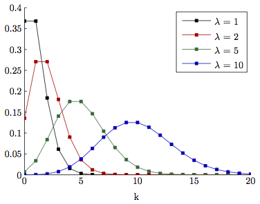
Figure 5: Siméon Denis Poisson and his distribution. (A) Poisson is said to have been extremely clumsy and uncoordinated with his hands. This contributed to him giving up an apprenticeship as a surgeon and entering mathematics, where the problem was less debilitating – although apparently this meant his diagrams tended not to very well drawn (see http://www-history.mcs.st-andrews.ac.uk/history/Biographies/Poisson.html). (B) The 'Probability Mass Function' of the Poisson distribution for several different values of λ. This allows one to see for any 'true signal' λ the probability of actually counting any actual value k. Although it is more likely that one will count exactly k = λ than any other possible k, as λ increases the probability of getting precisely this value becomes smaller and smaller.

Suppose that, on average, a single photon will be emitted from some part of a fluorescing sample within a particular time interval. The randomness entails that we cannot say for sure what will happen on any one occasion when we look; sometimes one photon will be emitted, sometimes none, sometimes two, occasionally even more. What we are really interested in, therefore, is not precisely how many photons are emitted, which varies, but rather the rate at which they would be emitted under fixed conditions, which is a constant. The difference between the number of photons actually emitted and the true rate of emission is the photon noise. The trouble is that keeping the conditions fixed might not be possible: leaving us with the problem of trying to figure out rates from single, noisy measurements.

Signal-dependent noise

Clearly, since it is a rate that we want, we could get that with more accuracy if we averaged many observations – just like with Gaussian noise, averaging reduces photon noise. Therefore, we can expect smoothing filters to work similarly for both noise types - and they do.

The primary distinction between the noise types, however, is that Poisson noise is signal-dependent, and does change according to the number of emitted (or detected) photons. Fortunately, the relationship is simple: if the rate of photon emission is $\lambda$ , the noise variance is also $\lambda$ , and the noise standard deviation is $\sqrt{\lambda}$ .

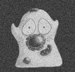
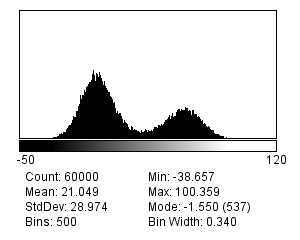
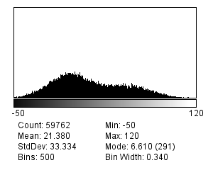
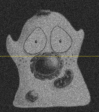
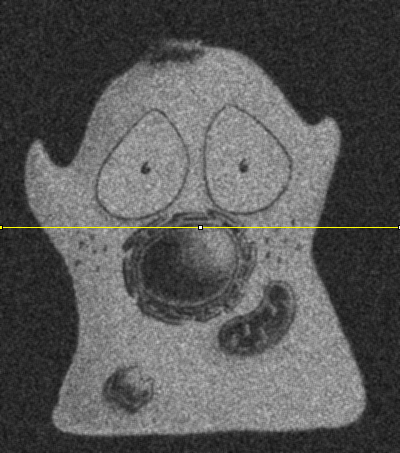
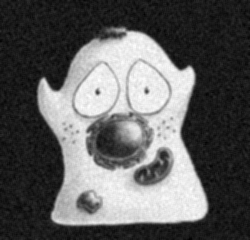
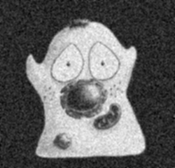
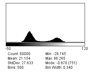
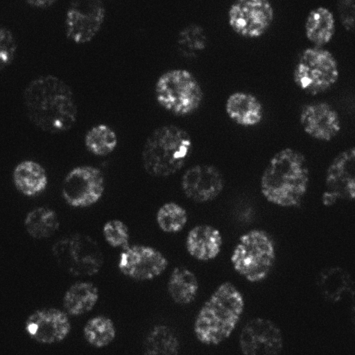
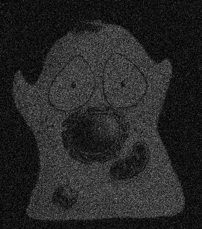
This is not really as unexpected as it might first seem (see Figure 6). It can even be observed from a very close inspection of Figure 7, in which the increased variability in the yeast cells causes their ghostly appearance even in an image that ought to consist only of noise.

Figure 6: 'The standard deviation of photon noise is equal to the square root of the expected value.' To understand this better, it may help to imagine a fisherman, fishing many times at the same location and under the same conditions. If he catches 10 fish on average, it would be quite reasonable to catch 7 or 13 on any one day – while 20 would be exceptional. If, however, he caught 100 on average, then it would be unexceptional if he caught 90 or 110 on a particular day, although catching only 10 would be strange (and presumably disappointing). Intuitively, the range of values that would be considered likely is related to the expected value. If nothing else, this imperfect analogy may at least help remember the name of the distribution that photon noise follows.

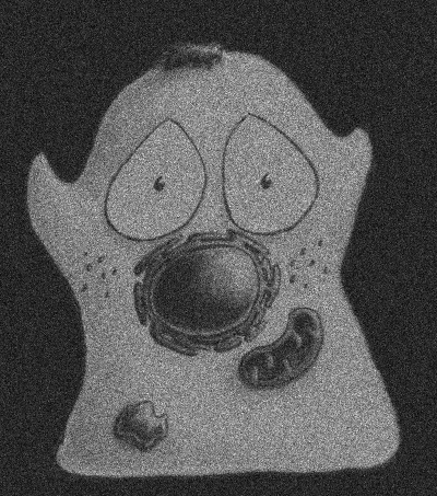
A: Original image

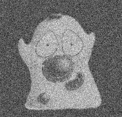
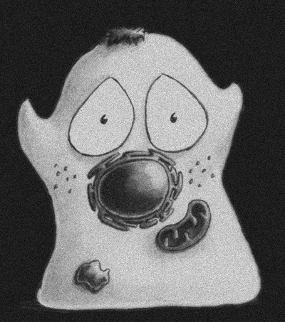
B: Gaussian filtered image

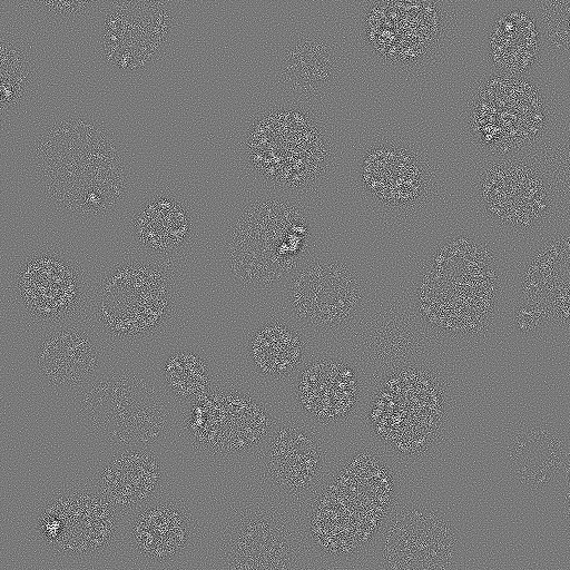
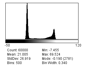
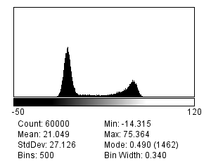
C: Result of (A) - (B)

Figure 7: A demonstration that Poisson noise changes throughout an image. (A) Part of a spinning disk microscopy image of yeast cells. (B) A Gaussian filtered version of (A). Gaussian filtering reduces the noise in an image by replacing each pixel with a weighted average of neighboring pixels (see Filters). (C) The difference between the original and filtered image contains the noise that the filtering removed. However, the locations of the yeast cells are still visible in this 'noise image' as regions of increased variability. This is partly an effect of Poisson noise having made the noise standard deviation larger in the brighter parts of the acquired image.

Question

The formula for the probability mass function of the Poisson distribution is:

$\mathcal{P}(\lambda) \sim \frac{e^{-\lambda}\lambda^{k}}{k!}$

where

$\lambda$ is the mean rate of occurrence of the event (i.e. the noise-free photon emission rate we want)
$k$ is an actual number of occurrences for which we want to compute the probability
$k!$ is the factorial of $k$ (i.e. $k \times (k-1) \times (k-2) \times ... \times 1$ )

So if you know that the rate of photon emission is 0.5, for example, you can put $\lambda = 0.5$ into the equation and determine the probability of getting any particular (integer) value of $k$ photons. Applying this, the probability of not detecting any photons ( $k = 0$ ) is 0.6065, while the probability of detecting a single photon ( $k = 1$ ) is $0.3033$ .

Assuming the mean rate of photon emission is 1, use the formula for the Poisson distribution probability mass function to calculate the probability of actually detecting 5 (which, at 5 times the true rate, would be an extremely inaccurate result). How common do you suppose it is to find pixels that are so noisy in the background region of a dark image?

Answer

The probability of detecting 5 photons is approximately 0.0031.

$\frac{e^{-1}}{5!} = \frac{1}{120e} = 0.0031$

Although this is a very low probability, images contain so many pixels that one should expect to see such noisy values often. For example, in a rather dark and dull 512 × 512 pixel image in which the average photon emission rate is 1, we would expect 800 pixels to have a value of 5 – and two pixels even to have a value of 8. The presence of isolated bright or dark pixels therefore usually tells us very little indeed, and it is only by processing the image more carefully and looking at surrounding values that we can (sometimes) discount the possibility these are simply the result of noise.

The SNR for Poisson noise

If the standard deviation of noise was the only thing that mattered, this would suggest that we are better not detecting much light: then photon noise is lower. But the SNR is a much more reliable guide. For noise that follows a Poisson distribution this is particularly easy to calculate. Substituting into the formula for the SNR

$\textrm{SNR}_{Poiss} = \frac{\lambda}{\sqrt{\lambda}} = \sqrt{\lambda}$

Therefore the SNR of photon noise is equal to the square root of the signal! This means that as the average number of emitted (and thus detected) photons increases, so too does the SNR. More photons → a better SNR, directly leading to the assertion

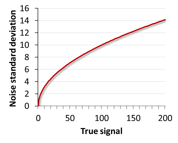
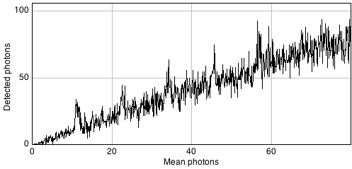
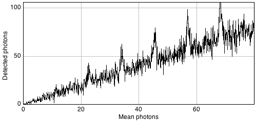
If you want to reduce photon noise, you need to detect more photons

A: Noise standard deviation

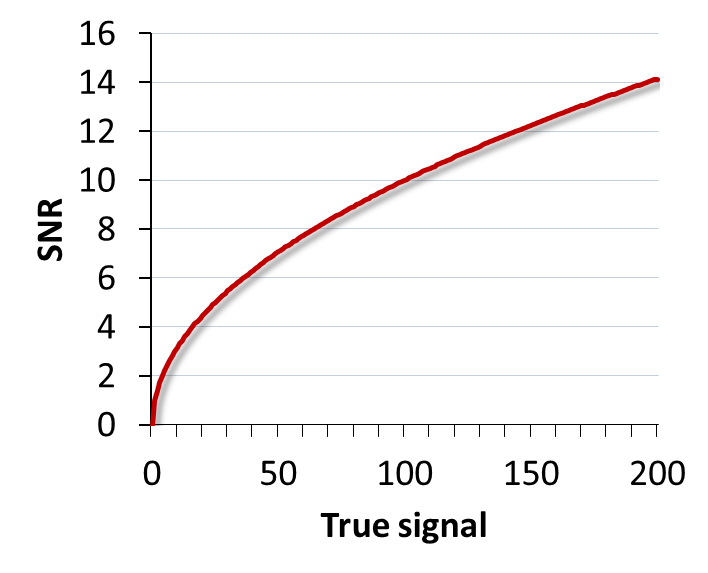
B: SNR

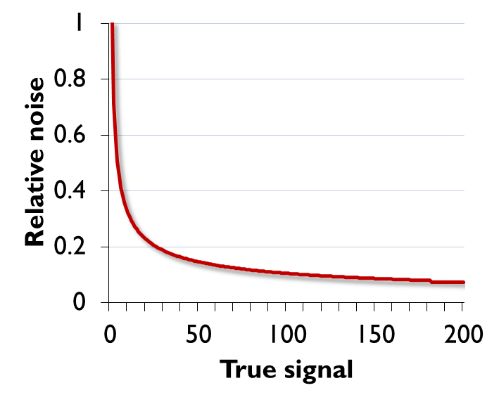
C: Relative noise

Figure 8: For Poisson noise, the standard deviation increases with the square root of the signal. So does the SNR, with the result that plots (A) and (B) look identical. This improvement in SNR despite the growing noise occurs because the signal is increasing faster than the noise, and so the noise is relatively smaller. Plotting the relative noise (1/SNR) shows this effect (C).

Why relativity matters: a simple example

The SNR increases with the number of photons, even though the noise standard deviation increases too, because it is really relative differences in the brightness in parts of the image that we are interested in. Absolute numbers usually are of very little importance – which is fortunate, since not all photons are detected.

Yet if you remain unconvinced that the noise variability can get bigger while the situation gets better, the following specific example might help. Suppose the true signal for a pixel is 4 photons. Assuming the actual measured value is within one noise standard deviation of the proper result (which it will be, about 68% of the time), one expects it to be in the range 2–6. The true signal at another pixel is twice as strong – 8 photons – and, by the same argument, one expects to measure a value in the range 5–11. The ranges for both pixels overlap! With photon counts this low, even if the signal doubles in brightness, we often cannot discern with confidence that the two pixels are even different at all. In fact, it is quite possible that the second pixel gives a lower measurement than the first.

On the other hand, suppose the true signal for the first pixel is 100 photons, so we measure something in the range of 90–110. The second pixel, still twice as bright, gives a measurement in the range 186–214. These ranges are larger, but crucially they are not even close to overlapping, so it is very easy to tell the pixels apart. Thus the noise standard deviation alone is not a very good measure of how noisy an image is. The SNR is much more informative: the simple rule is that higher is better. Or, if that still does not feel right, you can turn it upside down and consider the noise-to-signal ratio (the relative noise), in which case lower is better (Figure 8).

Poisson noise & detection

So why should you care that photon noise is signal-dependent?

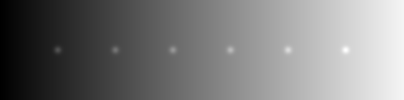
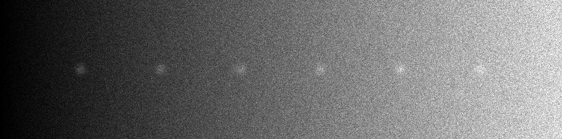
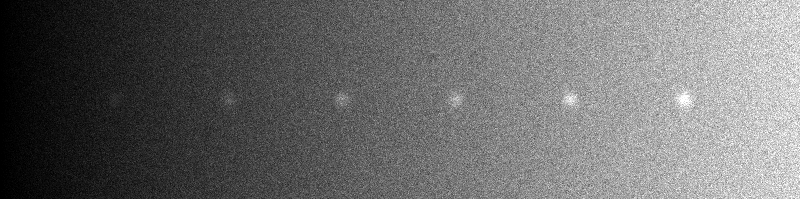
One reason is that it can make features of identical sizes and brightnesses easier or harder to detect in an image purely because of the local background. This is illustrated in Figure 9.

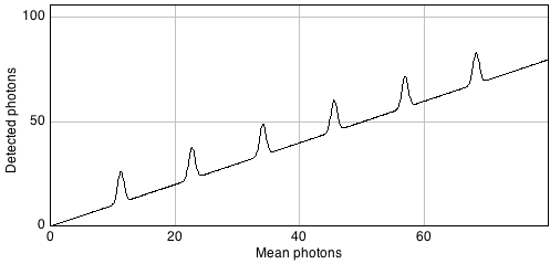
A: Seeing spots with the same absolute brightness

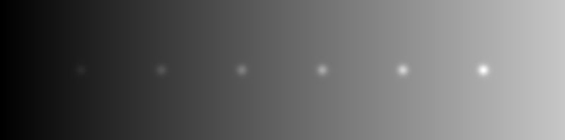
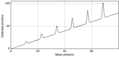
B: Seeing spots with the same relative brightness

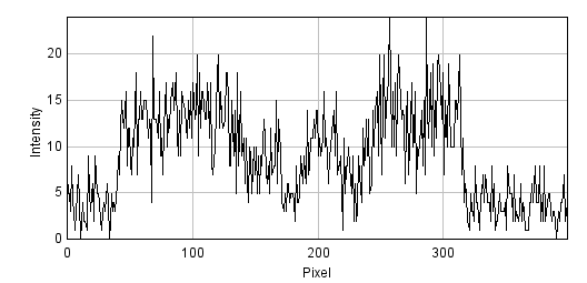
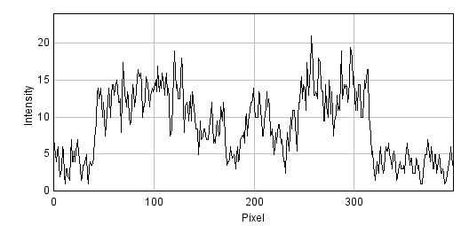
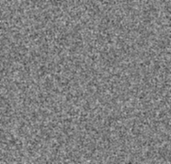
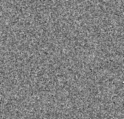
Figure 9: The signal-dependence of Poisson noise affects how visible (and therefore detectable) structures are in an image. (A) Six spots of the same absolute brightness are added to an image with a linearly increasing background (top) and Poisson noise is added (bottom). Because the noise variability becomes higher as the background increases, only the spots in the darkest part of the image can be clearly seen in the profile. (B) Spots of the same brightness relative to the background are added, along with Poisson noise. Because the noise is relatively lower as the brightness increases, now only the spots in the brightest part of the image can be seen.

In general, if we want to see a fluorescence increase of a fixed number of photons, this is easier to do if the background is very dark. But if the fluorescence increase is defined relative to the background, it will be much easier to identify if the background is high. Either way, when attempting to determine the number of any small structures in an image, for example, we need to remember that the numbers we will be able to detect will be affected by the background nearby. Therefore results obtained from bright and dark regions might not be directly comparable.

Simulating photon noise

If you install the RandomJ set of plugins^[4], you can add simulated Poisson noise to an image using Process ▸ Noise ▸ RandomJ ▸ RandomJ Poisson. The pixel values before adding the noise will be treated as the true signal if you select Insertion: modularity, in which case the choice of Mean setting does not matter.

Practical

Open the images mystery_noise_1.tif and mystery_noise_2.tif. Both are noisy, but in one the noise follows a Gaussian distribution (like read noise) and in the other it follows a Poisson distribution (like photon noise). Which is which?

Answer

The noise in mystery_noise_1.tif is Gaussian, it is Poisson in mystery_noise_2.tif. Since there are reasonably flat regions within the cell and background, I would test this by drawing a ROI within each and measuring the standard deviations. Where these are similar, the noise is Gaussian; if there is a big difference, the noise is likely to be Poisson.

If no flat regions were available, I would try applying a gradient filter with the coefficients -1 1 0, and inspecting the results. Alternatively, I might try plotting a fluorescence profile or subtracting a very slightly smoothed version of each image.

Combining noise sources

Combining our noise sources then, we can imagine an actual pixel value as being the sum of three values: the true rate of photon emission, the photon noise component, and the read noise component^[5]. The first of these is what we want, while the latter two are random numbers that may be positive or negative.

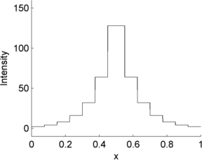
A: A noise-free signal

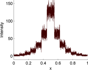
B: Photon noise

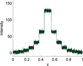
C: Read noise

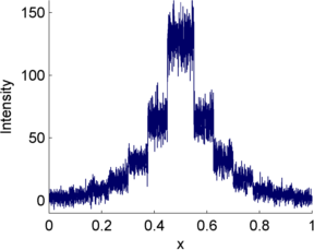
D: Photon + Read noise

Figure 10: An illustration of how photon noise differs from read noise. When both are added to a signal (here, a series of steps in which the value doubles at each higher step), the relative importance of each depends upon the value of the signal. At low signal levels this doubling is very difficult to discern amidst either type of noise, and even more so when both noise components are present.

This is illustrated in Figure 10 using a simple 1D signal consisting of a series of steps. Random values are added to this to simulate photon and read noise. Whenever the signal is very low (indicating few photons), the variability in the photon noise is very low (but high relative to the signal! (B)). This variability increases when the signal increases. However, in the read noise case (C), the variability is similar everywhere. When both noise types are combined in (D), the read noise dominates completely when there are few photons, but has very little impact whenever the signal increases. Photon noise has already made detecting relative differences in brightness difficult when there are few photons; with read noise, it can become hopeless.

Therefore overcoming read noise is critical for low-light imaging, and the choice of detector is extremely important (see Microscopes & detectors). But, where possible, detecting more photons is an extremely good thing anyway, since it helps to overcome both types of noise.

Other noise sources

Photon and read noise are the main sources of noise that need to be considered when designing and carrying out an experiment. One other source often mentioned in the literature is dark noise, which can be thought of as arising when a wayward electron causes the detector to register a photon even when there was not actually one there. In very low-light images, this lead to spurious bright pixels. However, dark noise is less likely to cause problems if many true photons are detected, and many detectors reduce its occurrence by cooling the sensor.

If the equipment is functioning properly, other noise sources could probably not be distinguished from these three. Nevertheless, brave souls who wish to know more may find a concise, highly informative, list of more than 40 sources of imprecision in The 39 steps: a cautionary tale of quantitative 3-D fluorescence microscopy by James Pawley (available online from various sources).

Question

Suppose you have an image that does not contain much light, but has some isolated bright pixels. Which ImageJ command could you use to remove them? And is it safe to assume they are due to dark noise or something similar, or might the pixels correspond to actual bright structures?

Answer

A median filter is a popular choice for removing isolated bright pixels, although I sometimes prefer Process ▸ Noise ▸ Remove Outliers… because this only puts the median-filtered output in the image if the original value was really extreme (according to some user-defined threshold). This then preserves the independence of the noise at all other pixels – so it still behaves reliably and predictably like Poisson + Gaussian noise. We can reduce the remaining noise with a Gaussian filter if necessary.

Assuming that the size of a pixel is smaller than the PSF (which is usually the case in microscopy), it is a good idea to remove these outliers. They cannot be real structures, because any real structure would have to extend over a region at least as large as the PSF. However if the pixel size is very large, then we may not be able to rule out that the 'outliers' are caused by some real, bright structures.

Finding photons

There are various places from which the extra photons required to overcome noise might come. One is to simply acquire images more slowly, spending more time detecting light. If this is too harsh on the sample, it may be possible to record multiple images quickly. If there is little movement between exposures, these images could be added or averaged to get a similar effect (Figure 11).

A: 1 image

B: 10 images

C: 100 images

D: 1000 images

Figure 11: The effect of adding (or averaging) multiple noisy images, each independent with a similar SNR.

An alternative would be to increase the pixel size, so that each pixel incorporates photons from larger regions – although clearly this comes at a cost in spatial information.

Nyquist sampling

Small pixels are needed to see detail, but also reduce the number of photons per pixel and thereby increase noise. However, Blur & the PSF has already argued that ultimately it is not pixel size, but rather the PSF that limits spatial resolution – which suggests that there is a minimum pixel size below which nothing is gained, and the only result is that more noise is added.

This size can be determined based upon knowledge of the PSF and the Nyquist-Shannon sampling theorem (Figure 12). Images acquired with this pixel size are said to be Nyquist sampled. The easiest way to determine the corresponding pixel size for a given experiment is to use the online calculator provided by Scientific Volume Imaging at http://www.svi.nl/NyquistCalculator. You may need larger pixels to reduce noise or see a wider field of view, but you do not get anything extra by using smaller pixels.

A: 50 x 50 pixels

B: 250 x 250 pixels

C: 500 x 500 pixels

Figure 12: Harry Nyquist (1889-1975) and Claude Shannon (1916-2001), sampled using different pixel sizes. Their work is used when determining the pixel sizes needed to maximize the available information when acquiring images, which depends upon the size of the PSF.

1. Specifically its probability density or mass function – which for a Gaussian distribution is the familiar bell curve.

2. Actually more. But the two mentioned here are usually by far the most significant, and it does not matter to our model at all if they contain various other sub-components. The important fact remains that there is some noise that varies throughout the image, and some that does not.

3. This is one definition of SNR. Many other definitions appear in the literature, leading to different values. The fact that any interesting image will vary in brightness in different places means that the SNR is not necessarily the same at all pixels – therefore computing it in practice involves coming up with some summary measurement for the whole image. This can be approached differently, but the general principle is always to compare how much noise we have relative to interesting things: where higher is better.

4. See https://imagescience.org/meijering/software/randomj/

5. For a fuller picture, gain and offset also need to be taken into consideration, see Microscopes & detectors.

Noise

Noise

Introduction

Background

Gaussian noise

Signal-to-Noise Ratio (SNR)

Gaussian noise simulations

Averaging noise

Poisson noise

Signal-dependent noise

The SNR for Poisson noise

Poisson noise & detection

Combining noise sources

Finding photons

results matching ""

No results matching ""