-
Filters can be used to reduce noise and/or enhance features, making detection & measurement much easier
-
Linear filters replace each pixel by a weighted sum of surrounding pixels
-
Nonlinear filters replace each pixel with the result of some other computation using surrounding pixels
-
Gaussian filters have various advantages that make them a good choice for many applications with fluorescence images
Filters
Chapter outline
Introduction
Filters are phenomenally useful. Almost all interesting image analysis involves filtering of some sort at some stage. In fact, the analysis of a difficult image sometimes becomes trivial once a suitable filter has been applied to it. It is therefore no surprise that much of the image processing literature is devoted to the topic of designing and testing filters.
The basic idea of filtering here is that each pixel in an image is assigned a new value depending upon the values of other pixels within some defined region (the pixel’s neighborhood). Different filters work by applying different calculations to the neighborhood to get their output. Although the plethora of available filters can be intimidating at first, knowing only a few of the most useful is already a huge advantage.
This chapter begins by introducing several extremely common linear and nonlinear filters for image processing. It ends by considering in detail some techniques based on one particularly important linear filter.
Linear filtering
Linear filters replace each pixel with a linear combination ('sum of products') of other pixels. Therefore the only mathematical background they require is the ability to add and multiply.
Mean filters
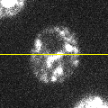
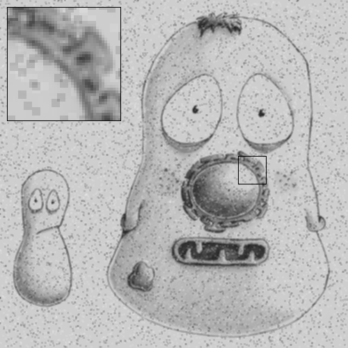
To begin, consider the somewhat noisy image of a yeast cell in Figure 1(A).
|

|
|
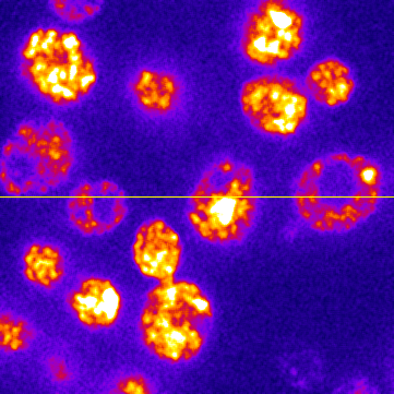
A: Original image
|
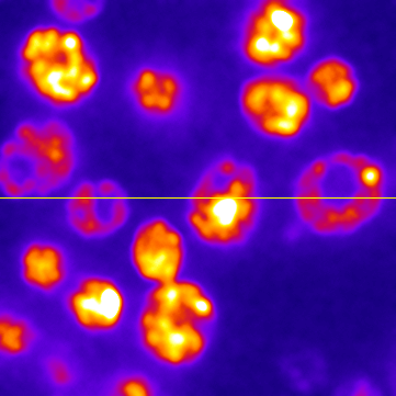
B: Mean filtered
|
C: Subtraction (A) - (B)
|
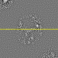
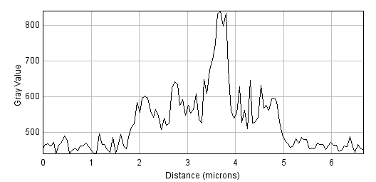
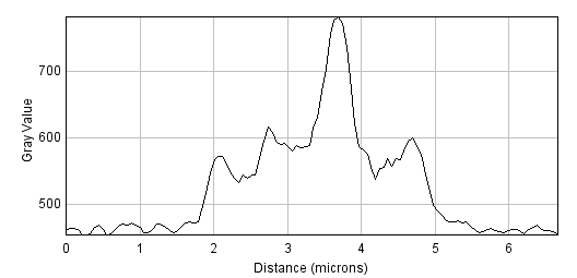
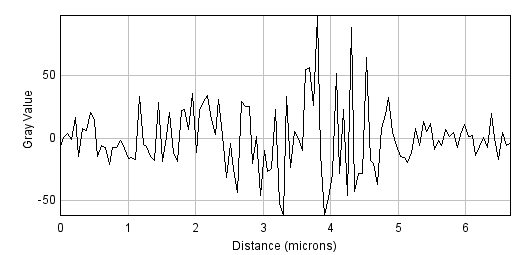
Figure 1: Filters can be used to reduce noise. A spinning disc confocal image of a yeast cell. Applying a small mean filter makes the image smoother, as is particularly evident in the fluorescence plot made through the image center. Computing the difference between images shows what the filter removed, which was mostly random noise.
The noise can be seen in the random jumps in the fluorescence intensity profile shown. One way to improve this is to take each pixel, and simply replace its value with the mean (average) of itself and the 8 pixels immediately beside it (including diagonals). This 'averages out' much of this noisy variation, giving a result that is considerably smoother (B). Subtracting the smoothed image from the original shows that what has been removed consists of small positive and negative values, mostly (but not entirely) lacking in interesting structure (C).
This smoothing is what a 3 × 3 mean filter[1] does. Each new pixel now depends upon the average of the values in a 3 × 3 pixel region: the noise is reduced, at a cost of only a little spatial information. The easiest way to apply this in ImageJ is through the command[2]. But this simple filter could be easily modified in at least two ways:
-
Its size could be increased. For example, instead of using just the pixels immediately adjacent to the one we are interested in, a 5 × 5 mean filter replaces each pixel by the average of a square containing 25 pixels, still centered on the main pixel of interest.
-
The average of the pixels in some other shape of region could be computed, not just an n × n square.
is ImageJ’s general command for mean
filtering. It uses approximately circular neighborhoods, and the
neighborhood size is adjusted by choosing a Radius value. The
Show Circular Masks command displays the neighborhoods used for
different values of Radius. If you happen to choose Radius = 1, you
get a 3 × 3 filter – and the same results as using
Smooth.

|
|
|
|
A: Original image
|
B: Filtered, radius=1
|
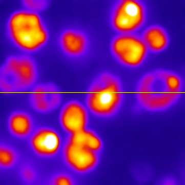
C: Filtered, radius=5
|
D: Filtered, radius=10
|
Figure 2: Smoothing an image using mean filters with different radii.
Figure 2 shows that as the radius increases, the image becomes increasingly smooth – losing detail along with noise. This causes the result to look blurry. If noise reduction is the primary goal, it is therefore best to avoid unnecessary blurring by using the smallest filter that gives acceptable results. More details on why mean filters reduce noise, and by how much, will be given in the chapter on Noise.
General linear filters
There are various ways to compute a mean of N different pixels. One is to add up all the values, then divide the result by N. Another is to multiply each value by 1/N, then add up the results. The second approach has the advantage that it is easy to modify to achieve a different outcome by changing the weights used to scale each pixel depending upon where it is. This is how a linear filter works in general, and mean filters are simply one specific example.
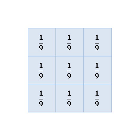
A: 3 × 3 square
|
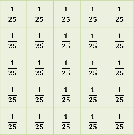
B: 5 × 5 square
|
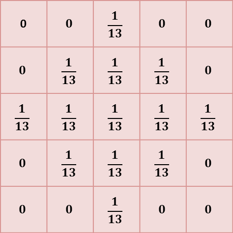
C: Circular, radius = 1.5
|
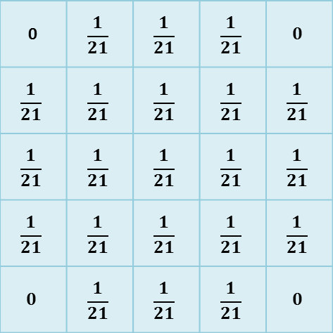
D: Circular, radius = 2
|
Figure 3:
The kernels used with several mean filters. Note that (C) and (D) are the 'circular' filters used by ImageJ’s Mean… command for different radii.
A linear filter is defined by a filter kernel (or filter mask). This resembles another (usually small and rectangular) image in which each pixel is known as a filter coefficient and these correspond to the the weights used for scaling. In the case of a mean filter, the coefficients are all the same (or zero, if the pixel is not part of the neighborhood), as shown in Figure 3. But different kernels can give radically different results, and be designed to have very specific properties.
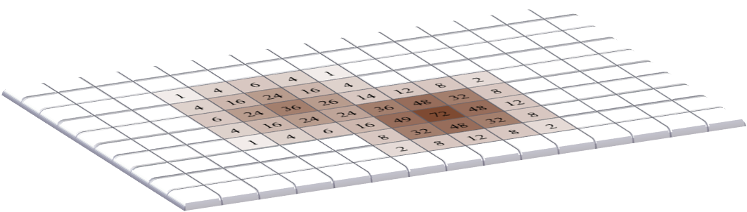
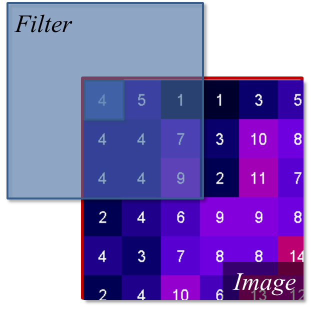
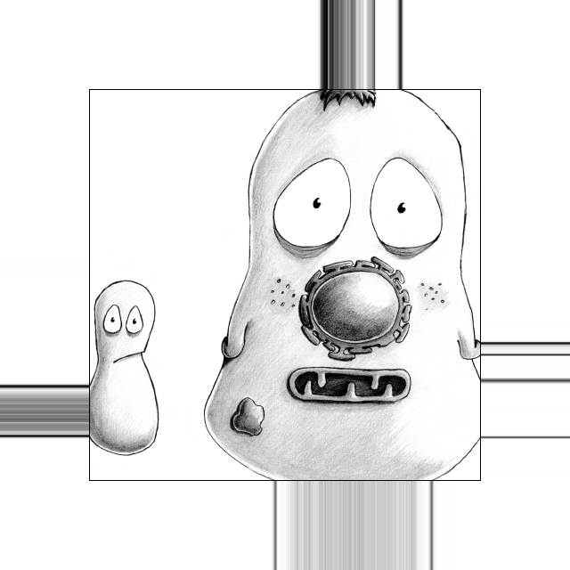
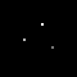
An algorithm to apply the filtering is shown in Figure 4.
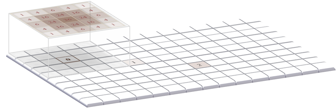
A: The filter is positioned over the top corner of the image. The products of the filter coefficients and the corresponding image pixel values are added together, and the result inserted in a new output image (although here the output is displayed in the original image to save space).
|
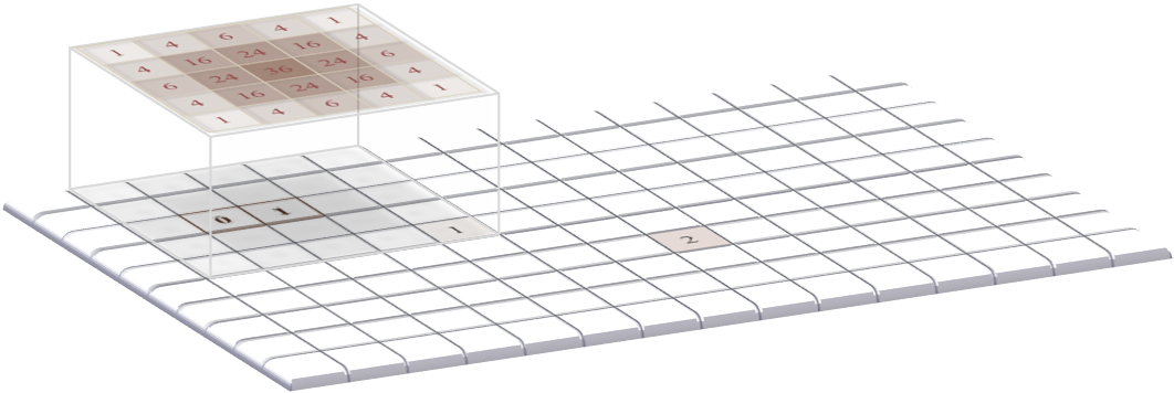
B: The filter is shifted to the next pixel in line, and the process repeated.
|
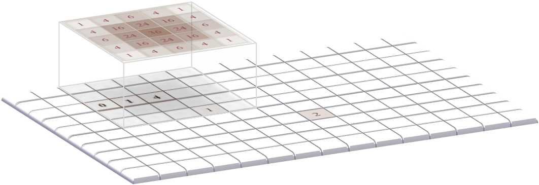
C: The filtering continues into the third pixel.
|
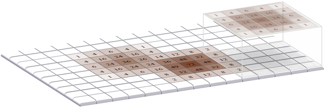
D: The filtering operation is applied to all pixels in the image to produce the final output.
|
Figure 4: Applying a linear filter to an image containing two non-zero pixels using the sum-of-products algorithm. The result is an image that looks like it contains two (scaled) versions of the filter itself, which in this case overlap with one another.
Defining your own filters
The application of such filtering is often referred to as convolution,
and if you like you can go wild inventing your own filters using the
command. This allows you to choose
which specific coefficients the filter should have, arranged in rows and
columns. If you choose the Normalize Kernel option then the
coefficients are scaled so that they add to 1 (if possible), by dividing
by the sum of all the coefficients.
Gradient filters
Often, we want to detect structures in images that are distinguishable from the background because of their edges. So if we could detect the edges we would be making good progress. Because an edge is usually characterized by a relatively sharp transition in pixel values – i.e. by a steep increase or decrease in the profile across the image – gradient filters can be used to help.
A very simple gradient filter has the coefficients -1, 0, 1. Applied
to an image, this replaces every pixel with the difference between the
pixel to the right and the pixel to the left. The output is positive
whenever the fluorescence is increasing horizontally, negative when the
fluorescence is decreasing, and zero if the fluorescence is constant –
no matter what the original constant value was, so that flat areas are
zero in the gradient image irrespective of their original brightness. We
can also rotate the filter by 90 and get a vertical gradient image
(Figure 5).
A: Horizontal gradient
|
B: Vertical gradient
|
C: Gradient magnitude
|
Figure 5: Using gradient filters and the gradient magnitude for edge enhancement.
Having two gradient images with positive and negative values can be somewhat hard to work with. If we square all the pixels in each, the values become positive. Then we can add both the horizontal and vertical images together to combine their information. If we compute the square root of the result, we get what is known as the gradient magnitude[3], which has high values around edges, and low values everywhere else. This is (almost) what is done by the command .
Convolution & correlation
Although linear filtering and convolution are terms that are often used synonymously, the former is a quite general term while the latter can be used in a somewhat more restricted sense. Specifically, for convolution the filter should be rotated by 180 before applying the algorithm of Figure 4. If the algorithm is applied without the rotation, the result is really a correlation. However, this distinction is not always kept in practice; convolution is the more common term, and often used in image processing literature whenever no rotation is applied. Fortunately, much of the time we use symmetric filters, in which case it makes absolutely no difference which method is used. But for gradient filters, for example, it is good to be aware that the sign out the output (i.e. positive or negative) would be affected.
Why rotate a filter for convolution?
It may not be entirely clear why rotating a filter for convolution would be worthwhile. One partial explanation is that if you convolve a filter with an image containing only a single non-zero pixel that has a value of one, the result is an exact replica of the filter. But if you correlate the filter with the same image, the result is a rotated version of the filter. This can be inferred from Figures 4A and 4B: you can see that when the bottom right value of the filter overlaps with the first non-zero pixel, it results in the filter coefficient’s value being inserted in the top left of the image. Thus the application of the algorithm in Figure 4 inherently involves a rotation, and by rotating the filter first this is simply 'corrected'.
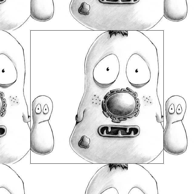
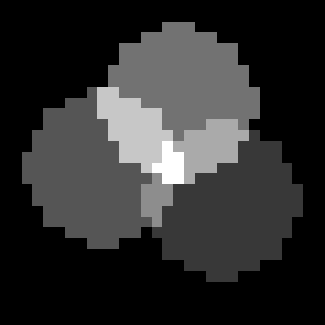
This leads to an equivalent way to think of convolution: each pixel value in an image scales the filter, and then these scaled filters replace the original pixels in the image – with overlapping values added together (Figure 6). This idea reappears in Blur & the PSF, because convolution happens to also describe the blur inherent in light microscopy.
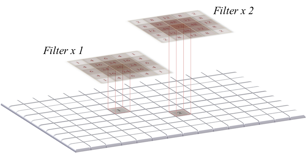
A: A copy of the filter is centered on every non-zero pixel in the image, and its coefficients are multiplied by the value of that pixel.
|
B: The coefficients of the scaled filters are assigned to the pixels of the output image, and overlapping values added together.
|
Figure 6: An alternative view of convolution as the summation of many scaled filters. Here, only two pixels in the original image have non-zero values so only two copies of the filter are needed, but often all pixels are non-zero – resulting in the addition of as many scaled filters as there are pixels. The final image computed this way is the same as that obtained by the method in Figure 4 – assuming either symmetrical filters, or that one of them has been rotated.
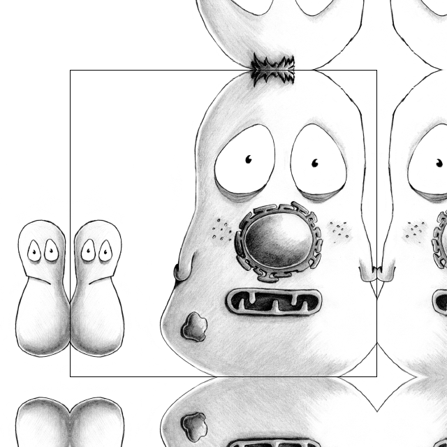
Filtering at image boundaries
 If a filter consists of more than one coefficient, the neighborhood
will extend beyond the image boundaries when filtering some pixels
nearby. These boundary pixels could simply be ignored and left with
their original values, but for large neighborhoods this would result in
much of the image being unfiltered. Alternative options include treating
every pixel beyond the boundary as zero, replicating the closest valid
pixel, treating the image as if it is part of a periodic tiling, or
mirroring the internal values (Figure 7).
If a filter consists of more than one coefficient, the neighborhood
will extend beyond the image boundaries when filtering some pixels
nearby. These boundary pixels could simply be ignored and left with
their original values, but for large neighborhoods this would result in
much of the image being unfiltered. Alternative options include treating
every pixel beyond the boundary as zero, replicating the closest valid
pixel, treating the image as if it is part of a periodic tiling, or
mirroring the internal values (Figure 7).
A: Original image
|
B: Zeros
|
C: Replication
|
D: Zeros
|
E: Replication
|
Figure 7: Methods for determining suitable values for pixels beyond image boundaries when filtering.
Nonlinear filters
Linear filters involve taking neighborhoods of pixels, scaling them by specified constants, and adding the results to get new pixel values. Nonlinear filters also make use of neighborhoods of pixels, but with different calculations to obtain the output. Here we will consider one especially important family of nonlinear filters.
Rank filters
Rank filters effectively sort the values of all the neighboring pixels in ascending order, and then choose the output based upon this ordered list. The most common example is the median filter, in which the pixel value at the center of the list is used for the filtered output.
Figure 8: Results of different 3 × 3 rank filters when processing a single neighborhood in an image. The output of a 3 × 3 mean filter in this case would also be 15.
The result of applying a median filter is often similar to that of applying a mean filter, but has the major advantage of removing extreme isolated values completely, without allowing them to have an impact upon surrounding pixels. This is in contrast to a mean filter, which cannot ignore extreme pixels but rather will smooth them out into occupying larger regions (Figure 9). However, a disadvantage of a median filter is that it can seem to introduce patterns or textures that were not present in the original image, at least whenever the size of the filter increases (see Figure 13D). Another disadvantage is that large median filters tend to be slow.
A: Mean filter
|

B: Median filter
|
Figure 9: Applying mean and median filters (radius = 1 pixel) to an image containing isolated extreme values (known as salt and pepper noise). A mean filter reduces the intensity of the extreme values but spreads out their influence, while a small median filter is capable of removing them completely with a minimal effect upon the rest of the image.
Other rank filters include the minimum and maximum filters, which replace each pixel value with the minimum or maximum value in the surrounding neighborhood respectively (Figure 10). They will become more important when we discuss Binary images.
A: Median filter
|
B: Maximum filter
|
C: Minimum filter
|
Figure 10: The result of applying three rank filters (radius = 1 pixel) to the noise-free image in Figure 13A.
Gaussian filters
Gaussian filters from Gaussian functions
We end this chapter with one fantastically important linear filter, and some variants based upon it. A Gaussian filter is a linear filter that also smooths an image and reduces noise. However, unlike a mean filter – for which even the furthest away pixels in the neighborhood influence the result by the same amount as the closest pixels – the smoothing of a Gaussian filter is weighted so that the influence of a pixel decreases with its distance from the filter center. This tends to give a better result in many cases (Figure 11).
A: Original dots
|
B: Mean filtered
|
C: Gaussian filtered
|
Figure 11: Comparing a mean and Gaussian filter. The mean filter can introduce patterns and maxima where previously there were none. For example, the brightest region in (B) is one such maximum – but the values of all pixels in the same region in (A) were zero! By contrast, the Gaussian filter produced a smoother, more visually pleasing result, less prone to this effect (C).
The coefficients of a Gaussian filter are determined from a Gaussian
function (Figure 12), and its size is controlled by a
value – so when working with ImageJ’s
Gaussian Blur… command, you will need to specify this rather than
the filter radius. is equivalent to the standard
deviation of a normal (i.e. Gaussian) distribution.
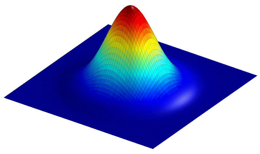
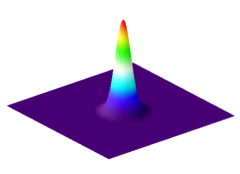
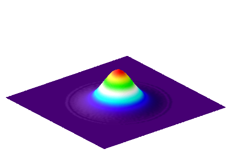
Figure 12: Surface plot of a 2D Gaussian function, calculated using the equation
The scaling factor is used to make the entire volume under the surface equal to 1, which in terms of filtering means that the coefficients add to 1 and the image will not be unexpectedly scaled. The size of the function is controlled by .
A comparison of several filters is shown in Figure 13.
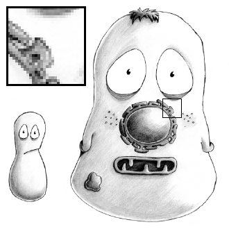
A: Original, noise-free image
|
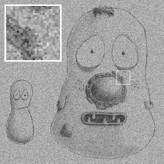
B: Noisy image
|
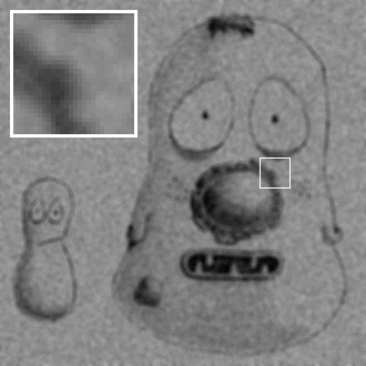
C: Mean filtered, radius = 2
|

D: Median filtered, radius = 2
|

E: Gaussian filtered,
|
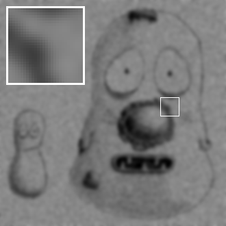
F: Gaussian filtered,
|
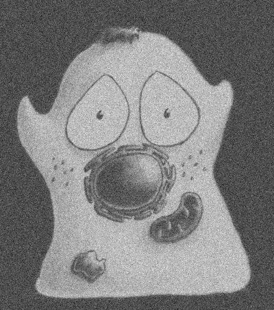
Figure 13: The effects of various linear and nonlinear filters upon a noisy image of a fixed cell.
Filters of varying sizes
Gaussian filters have useful properties that make them generally preferable to mean filters, some of which will be mentioned in Blur & the PSF (others require a trip into Fourier space, beyond the scope of this book). Therefore if in doubt regarding which filter to use for smoothing, Gaussian is likely to be the safer choice. Nevertheless, your decisions are not at an end since the size of the filter still needs to be chosen.
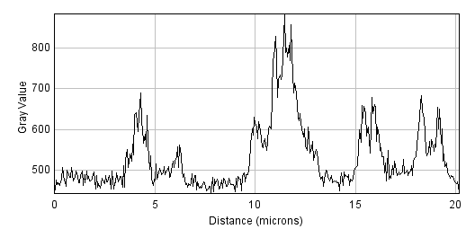
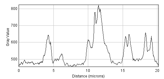
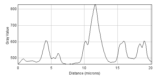
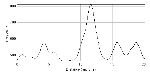
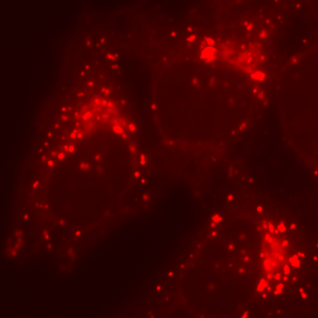
A small filter will mostly suppress noise, because noise masquerades as tiny fluorescence fluctuations at individual pixels. As the filter size increases, Gaussian filtering starts to suppress larger structures occupying multiple pixels – reducing their intensities and increasing their sizes, until eventually they would be smoothed into surrounding regions (Figure 14). By varying the filter size, we can then decide the scale at which the processing and analysis should happen.

A: Original image
|
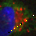
B: Gaussian
|
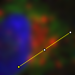
C: Gaussian
|
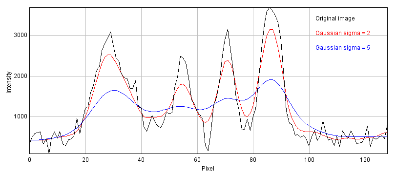
D: Profile plots of the intensity in the red channel of the image
|
||
Figure 14: The effect of Gaussian filtering on the size and intensity of structures. The image is taken from , with some additional simulated noise added to show that this is also reduced by Gaussian filtering.
Figure 15 shows an example of when this is useful. Here, gradient magnitude images are computed similar to that in Figure 5, but because the original image is now noisy the initial result is not very useful – with even strong edges being buried amid noise (B). Applying a small Gaussian filter prior to computing the gradient magnitude gives much better results (C), but if we only wanted the very strongest edges then a larger filter would be better (D).
A: Original image
|
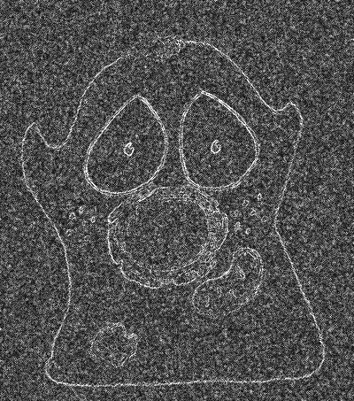
B: No smoothing
|
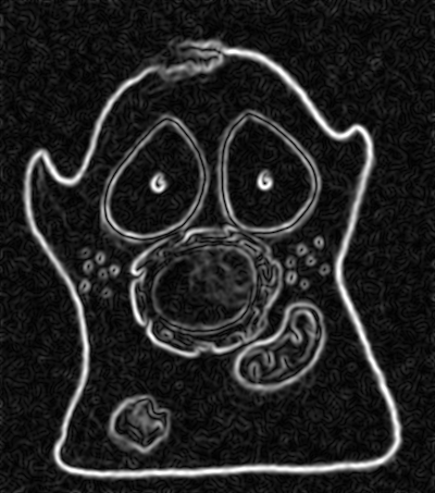
C: Gaussian
|
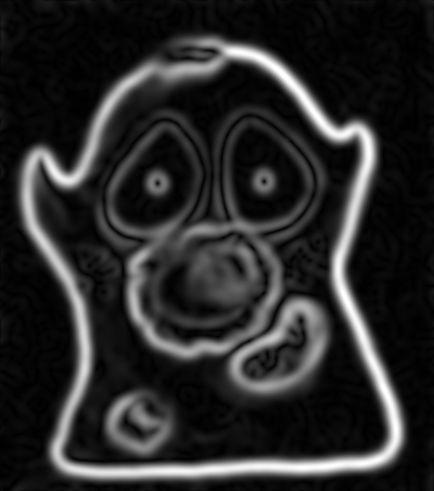
D: Gaussian
|
Figure 15: Applying Gaussian filters before computing the gradient magnitude changes the scale at which edges are enhanced.
Difference of Gaussians filtering
So Gaussian filters can be chosen to suppress small structures. But what if we also wish to suppress large structures – so that we can concentrate on detecting or measuring structures with sizes inside a particular range?
We already have the pieces necessary to construct one solution. Suppose we apply one Gaussian filter to reduce small structures. Then we apply a second Gaussian filter, bigger than the first, to a duplicate of the image. This will remove even more structures, while still preserving the largest features in the image. But if we finally subtract this second filtered image from the first, we are left with an image that contains the information that 'falls between' the two smoothing scales we used. This process is called difference of Gaussians (DoG) filtering, and it is especially useful for detecting small spots or as an alternative to the gradient magnitude for enhancing edges (Figure 16).
A: Original image
|
B: DoG, 1, 2
|
C: DoG, 2, 4
|
D: DoG, 4, 8
|
Figure 16: Difference of Gaussian filtering of the same image at various scales.
DoG filters
In fact, to get the result of DoG filtering it is not necessary to filter the image twice and subtract the results. We could equally well subtract the coefficients of the larger filter from the smaller first (after making sure both filters are the same size by adding zeros to the edges as required), then apply the resulting filter to the image only once (Figure 17).
A: Small Gaussian filter
|
B: Larger Gaussian filter
|
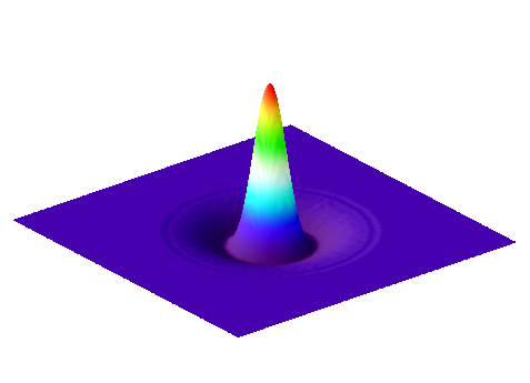
C: DoG filter
|
Figure 17: Surface plots of two Gaussian filters with small and large , and the result of subtracting the latter from the former. The sum of the coefficients for and is one in each case, while the coefficients of add to zero.
Laplacian of Gaussian filtering
One minor complication with DoG filtering is the need to select two different values of . A similar operation, which requires only a single and a single filter, is Laplacian of Gaussian (LoG) filtering. The appearance of a LoG filter is like an upside-down DoG filter (Figure 18), but if the resulting filtered image is inverted then the results are comparable[4]. You can test out LoG filtering in Fiji using [5].
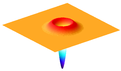
A: Laplacian of Gaussian filter
|
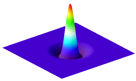
B: Inverted version of
|
Figure 18: Surface plot of a LoG filter. This closely resembles Figure 17, but inverted so that the negative values are found in the filter center.
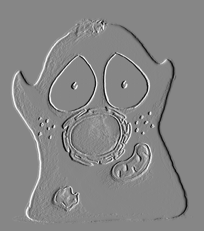
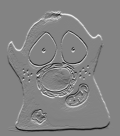
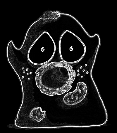
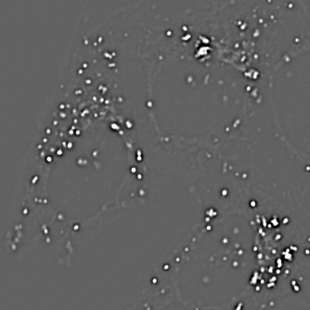
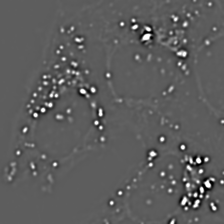
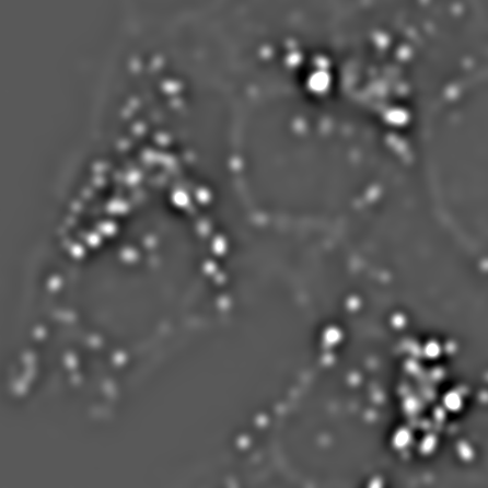
A: Original image
|
B: DoG filtered
|
C: LoG filtered
|
Figure 19: Application of DoG and LoG filtering to an image. Both methods enhance the appearance of spot-like structures, and (to a lesser extent) edges, and result in an image containing both positive and negative values with an overall mean of zero. In the case of LoG filtering, inversion is involved: darker points become bright after filtering.
Unsharp masking
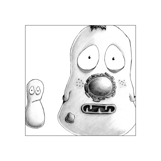
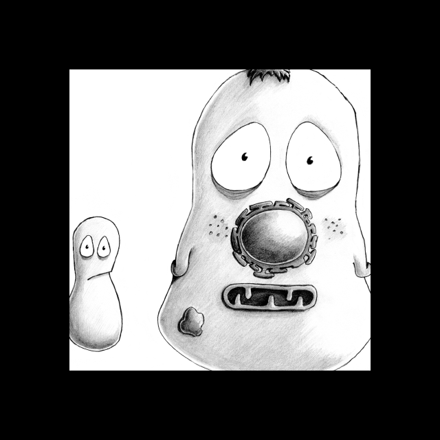
Finally, a related technique widely-used to enhance the visibility of details in images – although not advisable for quantitative analysis – is unsharp masking ().
This uses a Gaussian filter first to blur the edges of an image, and then subtracts it from the original. But rather than stop there, the subtracted image is multiplied by some weighting factor and added back to the original. This gives an image that looks much the same as the original, but with edges sharpened by an amount dependent upon the chosen weight.
A: Original image
|
B: Gaussian subtracted
|
C: Unsharp masked
|
Figure 20: The application of unsharp masking to a blurred image. First a Gaussian-smoothed version of the image () is subtracted from the original, scaled () and added back to the original.
Unsharp masking can improve the visual appearance of an image, but it is important to remember that it modifies the image content in a way that might well be considered suspicious in scientific circles. Therefore, if you apply unsharp masking to any image you intend to share with the world you should have a good justification and certainly admit what you have done. If you want a more theoretically justified method to improve image sharpness, it may be worth looking into '(maximum likelihood) deconvolution' algorithms.
1. Also called an arithmetic mean, averaging or box-car filter.
2. Note that the shortcut is Shift+S – a fact I rediscover regularly when intending to save my images. Be careful!
3. The equation then looks like Pythagoras' theorem:
4. A LoG filter is also often referred to as a mexican-hat filter, although clearly the filter (or the hat-wearer) should be inverted for the name to make more sense.
5. This now requires the use of a separate update site - see https://imagescience.org/meijering/software/featurej/ for installation information.