-
Image files consist of pixel values and metadata
-
Some file formats are suitable for data to analyze, others for data only to display
-
Metadata necessary for analysis can be lost by saving in a non-scientific file format
-
Compression can be either lossless or lossy
-
Original pixel values can be lost through lossy compression, conversion to RGB, or by removing dimensions
Files & file formats
Chapter outline
The contents of an image file
An image file stored on computer contains two main things:
-
Image data — the pixel values (numbers, only numbers)
-
Metadata — additional information, such as dimensions, image type, bit-depth, pixel sizes and microscope settings ('data about data')
The image data is clearly important. But some pieces of the metadata are essential for the image data to be interpretable at all. And if the metadata is incorrect or missing, measurements can also be wrong. Therefore files must be saved in formats that preserve both the pixel values and metadata accurately if they are to be suitable for analysis later.
File formats
When it comes to saving files, you have a choice similar to that faced when working with color images: you can either save your data in a file format good for analysis or good for display. The former requires a specialist microscopy/scientific format that preserves the metadata, dimensions and pixels exactly. For the latter, a general file format is probably preferable for compatibility.
Microscopy file formats (ICS, OME-TIFF, LIF, LSM, ND2…)
Fortunately, much useful metadata is normally available stored within freshly-acquired images. Unfortunately, this usually requires that the images are saved in the particular format of the microscope or acquisition software manufacturer (e.g. ND2 for Nikon, LIF or SCN for Leica, OIB or OIF for Olympus, CZI or ZVI for Zeiss). And it is quite possible that other software will be unable to read that metadata or, worse still, read it incorrectly or interpret it differently.
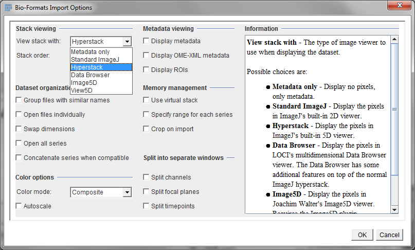
In Fiji, the job of dealing with most proprietary file formats is given to the LOCI Bioformats plugin[1]. This attempts to extract the most important metadata, and, if you like, can display its findings for you to check. When opening a file using Bioformats, the dialog box shown in Figure 1 appears first and gives some extra options regarding how you want the image to be displayed when it is opened.
|
Figure 1: Options when opening a file using the LOCI Bioformats importer.
In general, Bioformats does a very good job — but it does not necessarily get all the metadata in all formats. This is why…
The original files should be trustworthy most of the time. But it remains good to keep a healthy sense of paranoia, since complications can still arise: perhaps during acquisition there were values that ought to have been input manually (e.g. the objective magnification), without which the metadata is incorrect (e.g. the pixel size is miscalculated). This can lead to wrong information stored in the metadata from the beginning. So it is necessary to pay close attention at an early stage.
While in many cases an accurate pixel size is the main concern, other metadata can matter sometimes — such as if you want to estimate the blur of an image (see Blur & the PSF), and perhaps reduce it by deconvolution.
The messy state of metadata
Despite its importance, metadata can be annoyingly slippery and easy to lose. New proprietary file formats spring up, and the specifications for the formats might not be released by their creators, which makes it very difficult for other software developers to ensure the files are read properly.
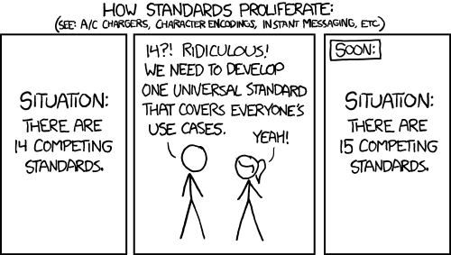
One significant effort to sort this out and offer a standardized format is being undertaken by the Open Microscopy Environment (OME), which is often encountered in the specific file format OME-TIFF. While such efforts give some room for hope, it has not yet won universal support among software developers.
General file formats (JPEG, PNG, MPEG, AVI, TIFF…)
If you save your data in a general format, it should be readable in a lot more software. However, there is a fairly good chance your image will be converted to 8-bit and/or RGB color, extra dimensions will be thrown away (leaving you with a 2D image only) and most metadata lost. The pixel values might also be compressed — which could be an even bigger problem.
Compression
There are two main categories of compression: lossy and lossless.
-
Lossy compression (e.g. JPEG) saves space by 'simplifying' the pixel values, and converting them into a form that can be stored more concisely. But this loses information, since the original values cannot be perfectly reconstructed. It may be fine for photographs if keeping the overall appearance similar is enough, but is terrible for any application in which the exact values matter.
-
Lossless compression (e.g. PNG, BMP, most types of TIFF, some microscopy formats) saves space by encoding the patterns in the image more efficiently, but in such a way that the original data can be perfectly reconstructed. No information is lost, but the reductions in file size are usually modest.
Therefore lossless compression should not cause problems, but lossy compression really can. The general rule is
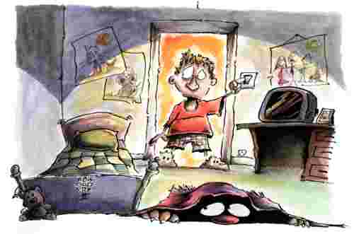
JPEG gets a special mention because it is ubiquitous, and its effects can be particularly ugly (Figure 2). It breaks an image up into little 8 × 8 blocks and then compresses these separately. Depending upon the amount of compression, you might be able to see these blocks clearly in the final image (Figure 3).
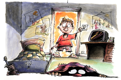
A: Uncompressed image (485 KB)
|
B: JPEG compressed image (10.3 KB)
|
Figure 2: The effect of strong JPEG compression on color images. The reduction in file size can be dramatic, but the changes to pixel values are irreversible. If you have an eerie sense that something might be wrong with an image, or the file size seems too good to be true, be sure to look closely for signs of little artificial square patterns that indicate that it was JPEG compressed once upon a time. By contrast, saving (A) as a PNG (which uses lossless compression) would give an image that looks identical to the original, but with a file size of 366 KB.

A: Uncompressed TIFF
|
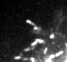
B: Compressed JPEG
|
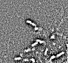
C: Subtracted TIFF
|
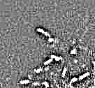
D: Subtracted JPEG
|
Figure 3: Using lossy compression can make some analysis impossible. The saved images in (A) and (B) look similar. However, after subtracting a smoothed version of the image, the square artifacts signifying the effects of JPEG compression are clearly visible in (D), but absent in (C). In later analysis of (B), it would be impossible to know the extent to which you are measuring compression artifacts instead of interesting phenomena.
File formats for creating figures
Preparing figures for publication can be a bewildering process. To begin with, it is necessary to make another distinction between image types, one of which has not been discussed here so far:
-
Bitmaps. These are composed of individual pixels: e.g. photographs, or all the microscopy images we are concerned with here.
-
Vector images. These are composed of lines, curves, shapes or text. The instructions needed to draw the image (i.e. coordinates, equations, fonts) are stored rather than pixels, and then the image is recreated from these instructions when necessary.
If you scale a 2D bitmap image by doubling its width and height, then it will contain four times as many pixels. Guesses need to be made about how to fill in the extra information properly (which is the problem of interpolation), and the result generally looks less sharp than the original. But if you double the size of a vector image, it is just a matter of updating the maths needed to draw the image accordingly, and the result looks just as sharp as the original.
Vector images are therefore best for things like diagrams, histograms, plots and charts, because they can be resized freely and still look good. Also, they often have tiny file sizes because only a few instructions to redraw the image need to be kept, whereas a huge number of pixels might be required to store sufficiently nice, sharp text in a bitmap. But bitmaps are needed for images formed from detecting light, which cannot be reduced to a few simple equations and instructions.
Finally, some versatile file formats, such as PDF or EPS, can store both kinds of image: perhaps a bitmap with some text annotations on top. If you are including text or diagrams, these formats are generally best. But if you only have bitmaps without annotations of any kind, then TIFF is probably the most common file format for creating figures.
A: Vector image or bitmap?
|
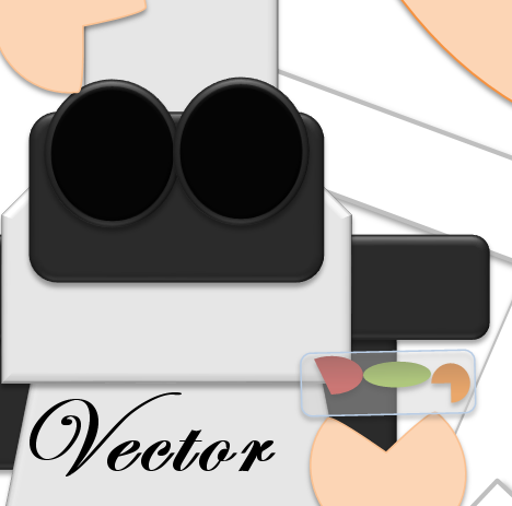
B: Enlargement of vector image
|
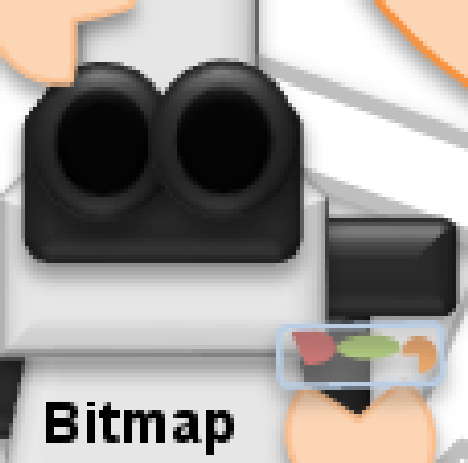
C: Enlargement of bitmap
|
Figure 4: When viewed from afar, it may be difficult to know whether an image is a vector or a bitmap (A) because they can sometimes look identical (although a photograph or micrograph will always be a bitmap). However, when enlarged a vector image will remain sharp (B), whereas a bitmap will not (C).
Choosing a file format
The table below summarizes the characteristics of some important file formats. Personally, I use ICS/IDS if I am moving files between analysis applications that support it (although you may well find OME-TIFF preferable, depending upon the software involved), and TIFF if I am just using ImageJ or Fiji. My favorite file format for most display is PNG[2], while I use PDF where possible for journal figures.
Dealing with large datasets
Large datasets are always troublesome, and we will not be considering datasets of tens or hundreds of gigabytes here. But when a file’s size is lurking beyond the boundary of what your computer can comfortably handle, one trick for dealing with this is to use a virtual stack.
Dimensions mentioned the (in practice often ignored) distinction between stacks and hyperstacks. Virtual stacks are a whole other idea. These provide a way to browse through large stacks or hyperstacks without needing to first read all the data into the computer’s memory. Rather, only the currently-displayed 2D image slice is shown. After moving the slider to look at a different time point, for example, the required image slice is read from its location on the hard disk at that moment. The major advantage of this is that it allows the contents of huge files to be checked relatively quickly, and it makes it possible to peek into datasets that are too large to be opened completely.
The disadvantage is that ImageJ can appear less responsive when browsing through a virtual stack because of the additional time required to access an image on the hard disk. Also, be aware that if you process an image that is part of a virtual stack, the processing will be lost when you move to view another part of the dataset!
Virtual stacks are set up either by or choosing the appropriate checkbox when the LOCI Bioformats plugin is used to open an image (see Figure 1).
Addendum: Whole slide images
The first part of this chapter was written at a time when I worked almost exclusively with fluorescence microscopy images. In this case, the message (as far as I was concerned) was clear: RGB images and JPEGs are bad, higher bit-depths are good, and virtual stacks can help with memory issues.
I then took up a new position working with whole slide images for digital pathology, for which none of the above is really true. In fact, the overwhelming majority of digital pathology images that I have encountered have been - from initial scanning - huge, JPEG-compressed RGB images that cannot even be opened as virtual stacks.
There are two main reasons for this:
-
Uncompressed whole slide scans are huge… often up to 40 GB for a single 2D plane.
-
Most (but not all) whole slide scans are brightfield, not fluorescence.
In general, brightfield images are inherently less suitable for quantitative analysis (based on intensity values) than fluorescence images. The more important issue in this case is to try to keep the data size at least somewhat manageable, and JPEG compression can at least reduce the file size from 40 GB image to around 1-2 GB. Therefore it is acceptable, even if it is not ideal, to use JPEG compression and work with RGB images. Nevertheless, other variations in compression (including JPEG 2000 or JPEG-XR) are becoming increasingly common for whole slide images, particularly for fluorescence applications.
With regards to analyzing such images, the fact that each 2D plane is so large causes considerable computational problems, and it is common to have to try to detect, measure and classify hundreds of thousands of cells across large tissue sections.
For this reason, I ended up writing new open source software for whole slide image analysis called QuPath, available at https://qupath.github.io. Naturally, QuPath integrates with ImageJ - so if you happen to want to try it out, whatever you might learn from this handbook could also be applied within QuPath as well.
Further documentation is provided at https://github.com/qupath/qupath/wiki.
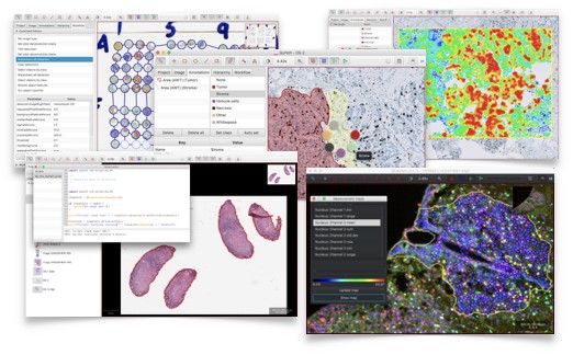
|
Figure 5: QuPath screenshots.
1. This can also be added to ImageJ, see http://loci.wisc.edu/software/bio-formats
2. If you ever email a Windows Bitmap file (BMP) to the sort of person who has a 'favorite file format', they will judge you for it, and possibly curse you for the time it takes to download. Unless, perhaps, that person was the designer of the BMP format. It is not well-compressed like JPEG or PNG, and nor does it contain much of the useful extra information a TIFF can store.