-
The choice of microscope influences the blur, noise & temporal resolution of images
-
An ideal detector would have a high Quantum Efficiency & low read noise
Microscopes & detectors
Chapter outline
Introduction
Successfully analyzing an image requires that it actually contains the necessary information in the first place. There are various practical issues related to the biology (e.g. not interfering too much with processes, such as by inadvertently killing things) and data handling (bit-depths, file formats, anything else in Part I of this handbook). However, assuming that these are in order, there are three other main factors to consider connected to the image contents:
-
Spatial information, dependent on the size and shape of the PSF,
-
Noise, dependent on the number of photons detected,
-
Temporal resolution, dependent on the speed at which the microscope can record images.
No one type of microscope is currently able to optimize all of these simultaneously, and so decisions and compromises need to be made. Temporal resolution and noise have an obvious relationship, in that a high temporal resolution means that less time is spent detecting photons in the image, leading to more photon noise. However, improving spatial information is also often related to one or both of the other two factors.
This chapter gives a very brief overview of the main features of several fluorescence microscopes from the point of view of how they balance the tradeoffs mentioned. Be aware that it does not do justice to all the complexities, variations and features of the microscopes it describes, and it is not written by an expert in microscopy - and therefore should be treated with some caution!
But it is included nonetheless in case it might be useful to anyone as a starting point[1].
Types of microscope

A: Widefield
|

B: LSCM
|

C: SDCM
|

D: 2-Photon
|

E: TIRF
|
Figure 1: Schematic diagrams to show the differences in excitation patterns. Here, an inverted microscope is assumed (the cell is resting on a coverslip, and illuminated from below). During the recording of a pixel, light can potentially be detected if it arises from any part of the green-illuminated region, although in the laser scanning and spinning disk confocal cases the pinhole will only permit a fraction of this light to pass through. Note that, for the 2-photon microscope, the excitation is confined to only the small, central region, while the red light above and below is not capable of exciting the fluorophores that have been used.
Widefield
So far, our schematic diagrams and PSF discussion (see Blur & the PSF) have concentrated on widefield microscopes. In widefield microscopy, the entire sample is bathed in light, so that many fluorophores throughout the sample can be excited and emit photons simultaneously. All of the light that enters the objective may then be detected and contribute to any image being recorded. Because photons are potentially emitted from everywhere in the sample, there will be a lot of blur present for a thick specimen (for a thin specimen there is not much light from out-of-focus planes because the planes simply do not contain anything that can fluoresce). What we get in any single recorded image is effectively the sum of the light from the in-focus plane, and every other out-of-focus plane. Viewed in terms of PSFs, we capture part of the hourglass shape produced by every light-emitting point depending upon how in-focus it is in every image.
This is bad news for spatial information and also for detecting small structures in thick samples, as the out-of-focus light is essentially background. On the other hand, widefield images tend to include a lot of photons, which overcomes read noise, even when they are recorded fast.
Laser scanning confocal
Optical sectioning is the ability to detect photons only from the plane of focus, rejecting those from elsewhere. This is necessary to look into thick samples without getting lost in the haze of other planes. Laser Scanning Confocal Microscopy (LSCM) achieves this by only concentrating on detecting light for one pixel at any time, and using a pinhole to try to only allow light from a corresponding point in the sample to be detected.
Because at most only one pixel is being recorded at any given moment, it does not make sense to illuminate the entire sample at once, which could do unnecessary damage. Rather, a laser illuminates only a small volume. If this would be made small enough, then a pinhole would not actually be needed because we would know that all emitted light must be coming from the illuminated spot; however, the illumination itself is like an hour-glass PSF in the specimen and so the pinhole is necessary to make sure only the light from the central part is detected. This then causes the final PSF, as it appears in the image, to take on more of a rugby-ball (or American football) appearance.
The end result is an image that has relatively little out-of-focus light. This causes a significant improvement in what can be seen along the z-dimension, although the xy resolution is not very different to the widefield case. Also, because single pixels are recorded separately, the image can (potentially) be more or less any size and shape – rather than limited by the pixel count on a camera.
However, these advantages comes with a major drawback. Images usually contain thousands to millions of pixels, and so only a tiny fraction of the time required to record an image is spent detecting photons for any one pixel in a LSCM image – unlike in the widefield case, where photons can be detected for all pixels over the entire image acquisition time. This can cause LSCM image acquisition to be comparatively slow, noisy (in terms of few detected photons) or both. Spatial information is therefore gained at a cost in noise and/or temporal resolution.
Spinning disk confocal
So a widefield system records all pixels at once without blocking the light from reaching the detector anywhere, whereas a LSCM can block out-of-focus light by only recording a single pixel at a time. Both options sound extreme: could there not be a compromise?
Spinning disk confocal microscopy (SDCM) implements one such compromise by using a large number of pinholes punched into a disk, so that the fluorophores can be excited and light detected for many different non-adjacent pixels simultaneously. By not trying to record adjacent pixels at the same time, pinholes can be used to block most of the out-of-focus light for each pixel, since this originates close to the region of interest for that pixel (i.e. the PSF becomes very dim at locations far away from its center) – but sufficiently-spaced pixels can still be recorded simultaneously with little influence on one another.
In practice, spinning disk confocal microscopy images are likely to be less sharp than laser scanning confocal images because some light does scatter through other pinholes. Also, the pinhole sizes cannot be adjusted to fine-tune the balance between noise and optical sectioning. However, the optical sectioning offered by SDCM is at least a considerable improvement over the widefield case, and an acceptable SNR can be achieved with much faster frame-rates using SDCM as opposed to LSCM.
Multiphoton microscopy
As previously mentioned, if the size of excitation volume could be reduced enough, then we would know where the photons originated even without a pinhole being required – but focused excitation is generally still subject to PSF-related issues, so that fluorophores throughout a whole hourglass-shaped volume can end up being excited. The main idea of multiphoton microscopy is that fluorophore excitation requires the simultaneous absorption of multiple photons, rather than only a single photon. The excitation light has a longer wavelength than would otherwise be required to cause molecular excitation with a single photon, but the energies of the multiple photons combine to cause the excitation.
The benefit of this is that the multiphoton excitation only occurs at the focal region of the excitation – elsewhere within the 'specimen PSF' the light intensities are insufficient to produce the 'multiphoton effect' and raise the fluorophores into an excited state. This means that the region of the specimen emitting photons at any one time is much smaller than when using single photon excitation (as in LSCM), and also less damage is being caused to the sample. Furthermore, multiphoton microscopy is able to penetrate deeper into a specimen – up to several hundred µm.
Total Internal Reflection Fluorescence
As previously mentioned, widefield images of very thin specimens do not suffer much from out-of-focus blur because light is not emitted from many other planes. Total Internal Reflection Fluorescence (TIRF) microscopy makes use of this by stimulating fluorescence only in a very thin section of the sample close to the objective. Very briefly, TIRF microscopy involves using an illumination angled so that the change in refractive index encountered by the light as it approaches the specimen causes a further change in angle sufficient to prevent the light from directly entering the specimen (i.e. it is 'totally internally reflected'). Nevertheless, fluorophores can still be excited by an evanescent wave that is produced when this occurs. This wave decays exponentially, so that only fluorophores right at the surface are excited – meaning fluorophores deeper within the specimen do not interfere with the recording.
Importantly, because the subsequent recording is essentially similar to that used when recording widefield images, photons are detected at all pixels in parallel and fast recording-rates are possible. Therefore if it is only necessary to see to a depth of about 100 nm, TIRF microscopy may be a good choice.
Photon detectors
Certain detectors are associated with certain types of microscopy, and differ according to the level and type of noise you can expect. Understanding the basic principles greatly helps when choosing sensible values for parameters such as gain, pixel size and binning during acquisition to optimize the useful information in the image. The following provides an very brief introduction to three common detectors.
PMTs: one pixel at a time
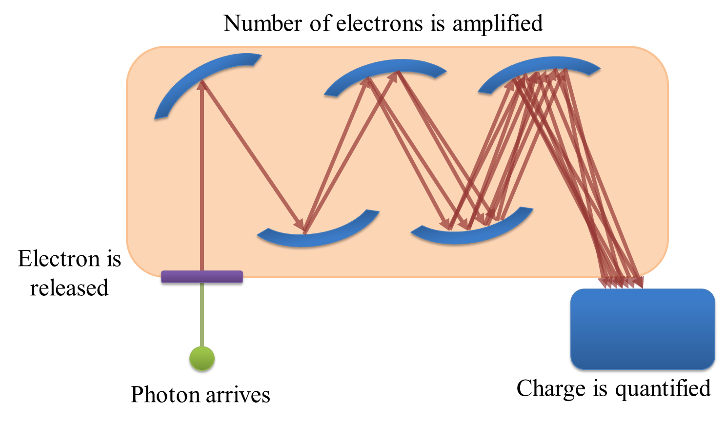
If you only need to record one pixel at a time, a photomultiplier tube (PMT) might be what you need. The basic principle is this: a photon strikes a photocathode, hopefully producing an electron. When this occurs, the electron is accelerated towards a dynode, and any produced electrons accelerated towards further dynodes. By adjusting the 'gain', the acceleration of the electrons towards successive dynodes can be varied; higher accelerations mean there is an increased likelihood that the collision of the electrons with the dynode will produce a higher number of electrons moving into the next stage. The charge of the electrons is then quantified at the end (Figure 2), but because the (possibly very small) number of original detected photons have now been amplified to a (possibly much) larger number electrons by the successive collisions with dynodes, the effect of read noise is usually minor for a PMT.
|
Figure 2: Diagram showing the detection of a photon by a PMT. Each photon can be 'multiplied' to produce many electrons by accelerating the first produced electron towards a dynode, and repeating the process for all electrons produced along a succession of dynodes. The charge of the electrons reaching the end of the process can then be quantified, and ought to be proportional to the number of photons that arrived at the PMT.
More problematically, PMTs generally suffer from the problem of having low quantum efficiencies (QEs). The QE is a measure of the proportion of photons striking the detector which then produce electrons, and typical values for a conventional PMT may be only 10–15%: the majority of the photons reaching the PMT are simply wasted. Thus photon noise can be a major issue, especially if there is a low amount of light available to detect in the first place.
CCDs: fast imaging when there are a lot of photons
A Charged Coupled Device (CCD) is a detector with a region devoted to sensing photons, and which is subdivided into different 'physical pixels' that correspond to pixels in the final image. Thus the image size cannot be changed arbitrarily, but it is possible to record photons for many pixels in parallel.
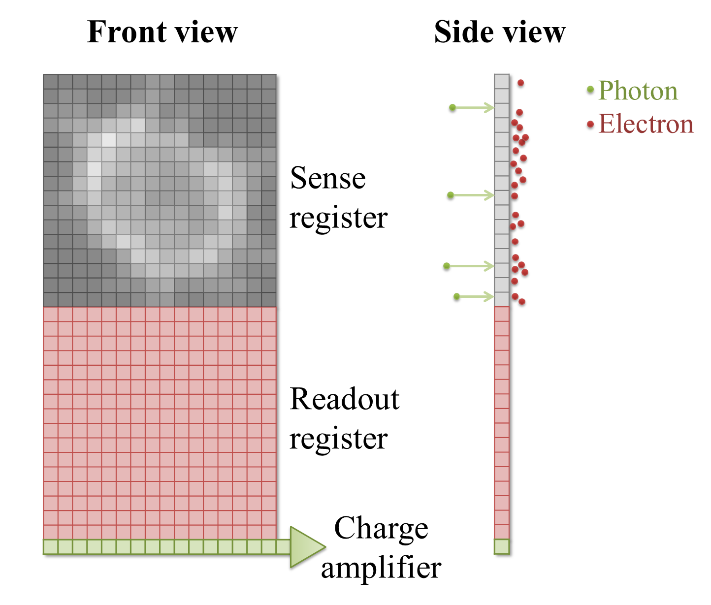
When a photon strikes a pixel in the sensing part of the CCD, this often releases an electron – the QE is typically high (perhaps 90%). After a certain exposure time, different 'electron clouds' have then formed at each physical pixel on the sensor, each of which has a charge related to the number of colliding photons. This charge is then measured by passing the electrons through a charge amplifier, and the results used to assign an intensity value to the pixel in the final image (Figure 3).
A: Photon detection
|
|||

B: Frame transfer
|
C: Quantification
|
||
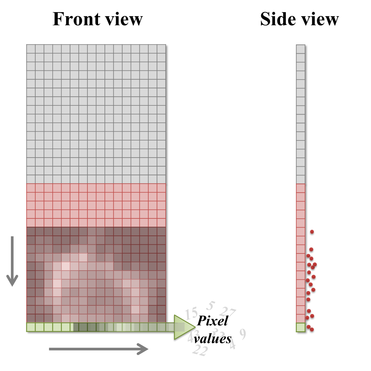
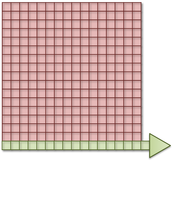
Figure 3: An illustration of the basic operation of a CCD camera (using frame transfer). First, photons strike a sense register, which is divided into pixels. This causes small clouds of electrons to be released and gather behind the pixels (A). These are then rapidly shifted downwards into another register of the same size, thereby freeing the sense register to continue detecting photons (B). The electron clouds are then shifted downwards again, one row at a time, with each row finally being shifted sequentially through a charge amplifier (C). This quantifies the charge of the electron clouds, from which pixel values for the final image are determined.
The electron clouds for each pixel might be larger than in the PMT case, both because of the higher QE and because more time can be spent detecting photons (since this is carried out for all pixels simultaneously). However, the step of amplifying the numbers of electrons safely above the read noise before quantification is missing. Consequently, read noise is potentially more problematic, and in some cases can even dominate the result.
Pixel binning
One way to address the issue of CCD read noise is to use pixel binning. In this case, the electrons from 4 (i.e. 2 × 2) pixels of the CCD are added together before being quantified: the electron clouds are approximately 4 times bigger relative to the read noise (Figure 4), and readout can be faster because fewer electron clouds need to be quantified. The obvious disadvantage of this is that one cannot then put the electrons from the 4 pixels 'back where they belong'. As a result, the binned measurement is simply treated as a single (bigger) pixel. The recorded image contains 25% of the pixels in the unbinned image, while still covering the same field of view, so spatial information is lost. Larger bins may also be used, with a correspondingly more dramatic impact upon image size (Figure 4D).
A: No binning
|
B: 2 × 2 binning
|
C: 4 × 4 binning
|

D: 8 × 8 binning
|
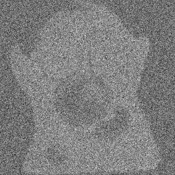
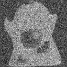
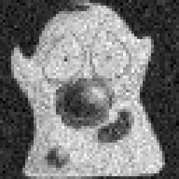
Figure 4: Illustration of the effect of binning applied to an image suffering from photon and read noise. As the bin size increases, the photons from neighboring pixels are combined into a single (larger) pixel before the read noise is added. As a consequence, the image becomes brighter relative to the read noise – but at a cost of spatial information.
EMCCDs: fast imaging with low light levels
And so you might wonder whether it is possible to increase the electron clouds (like with the PMT) with an CCD, and so get its advantages without the major inconvenience of read noise. Electron Multiplying CCDs (EMCCDs) achieve this to some extent. Here, the electrons are first passed through an additional 'gain register' before quantification. At every stage of this gain register, each electron has a small probability – perhaps only 1% – of being amplified (through 'impact ionisation') and giving rise to two electrons entering the next stage. Despite the small probability, by incorporating > 500 such stages, the size of the electron cloud arising from even a single photon may be amplified safely above the read noise.
However, the randomness of the amplification process itself introduces a new source of uncertainty, so that the final outcome can be thought of as having the same precision as if perhaps only around half as many photons were detected (see Noise for the relationship between noise and the number of photons). Therefore read noise is effectively overcome at the cost of more photon noise.
A: CCD (no binning)
|

B: CCD (2 × 2 binning)
|
C: EMCCD
|
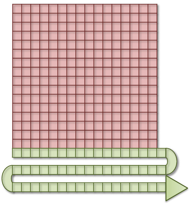
Figure 5: A simplified diagram comparing a conventional CCD (with and without binning) and an EMCCD. While each has the same physical number of pixels, when binning is used electrons from several pixels are combined before readout – thereby making the 'logical' pixels in the final image bigger. For the EMCCD, the electrons are shifted through a 'gain register' prior to quantification. See Figure 3 for additional labels; the sense register has been omitted for simplicity.
1. For a more extensive, and authoritative, description of the topics considered here, consider seeking out the Handbook of Biological Confocal Microscopy edited by James Pawley. This contains many excellent chapters, some of which may be freely available to download from the publisher’s website.