-
Measurements in fluorescence microscopy are affected by blur
-
Blur acts as a convolution with the microscope’s PSF
-
The size of the PSF depends on the microscope type, light wavelength & objective lens NA, and is on the order of hundreds of nm
-
In the focal plane, the PSF is an Airy pattern
-
Spatial resolution is a measure of how close structures can be distinguished. It is better in xy than along the z dimension.
Blur & the PSF
Chapter outline
Introduction
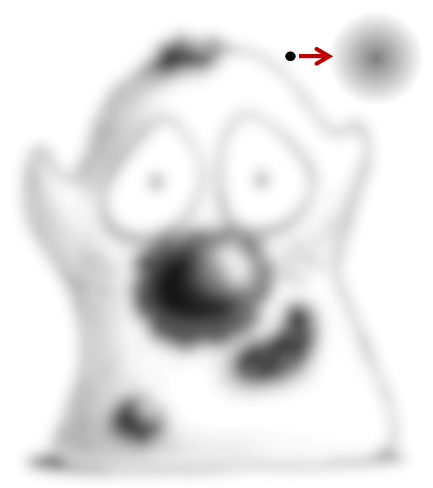
Microscopy images normally look blurry because light originating from one point in the sample is not all detected at a single pixel: usually it is detected over several pixels and z-slices. This is not simply because we cannot use perfect lenses; rather, it is caused by a fundamental limit imposed by the nature of light. The end result is as if the light that we detect is redistributed slightly throughout our data (Figure 1).

A: Sharp
|

B: Blurred
|
Figure 1: Schematic diagram showing the effects of blur. Think of the sand as photons, and the height of the sandcastle as the intensity values of pixels (a greater height indicates more photons, and thus a brighter pixel). The ideal data would be sharp and could contain fine details (A), but after blurring it is not only harder to discriminate details, but intensities in the brighter regions have been reduced and sizes increased (B). If we then wish to determine the size or height of one of the sandcastle’s towers, for example, we need to remember that any results we get by measuring (B) will differ from those we would have got if we could have measured (A) itself. Note, however, that approximately the same amount of signal (sand or photons) is present in both cases – only its arrangement is different.
This is important for three reasons:
-
Blur affects the apparent size of structures
-
Blur affects the apparent intensities (i.e. brightnesses) of structures
-
Blur (sometimes) affects the apparent number of structures
Therefore, almost every measurement we might want to make can be affected by blurring to some degree.
That is the bad news about blur. The good news is that it is rather well understood, and we can take some comfort that it is not random. In fact, the main ideas have already been described in Filters, because blurring in fluorescence microscopy is mathematically described by a convolution involving the microscope’s Point Spread Function (PSF). In other words, the PSF acts like a linear filter applied to the perfect, sharp data we would like but can never directly acquire.
Previously, we saw how smoothing (e.g. mean or Gaussian) filters could helpfully reduce noise, but as the filter size increased we would lose more and more detail. At that time, we could choose the size and shapes of filters ourselves, changing them arbitrarily by modifying coefficients to get the noise-reduction vs. lost-detail balance we liked best. But the microscope’s blurring differs in at least two important ways. Firstly, it is effectively applied to our data before noise gets involved, so offers no noise-reduction benefits. Secondly, because it occurs before we ever set our eyes on our images, the size and shape of the filter (i.e. the PSF) used are only indirectly (and in a very limited way) under our control. It would therefore be much nicer just to dispense with the blurring completely since it offers no real help, but unfortunately light conspires to make this not an option and we just need to cope with it.
The purpose of this chapter is to offer a practical introduction to why the blurring occurs, what a widefield microscope’s PSF looks like, and why all this matters. Detailed optics and threatening integrals are not included, although several equations make appearances. Fortunately for the mathematically unenthusiastic, these are both short and useful.
Blur & convolution
As stated above, the fundamental cause of blur is that light originating from an infinitesimally small point cannot then be detected at a similar point, no matter how great our lenses are. Rather, it ends up being focused to some larger volume known as the PSF, which has a minimum size dependent upon both the light’s wavelength and the lens being used.
A: Entire image
|
B: Detail of (A)
|
C: Some blur
|
D: A lot of blur
|
Figure 2: Images can be viewed as composed of small points (B), even if these points are not visible without high magnification (A). This gives us a useful way to understand what has happened in a blurred image: each point has simply been replaced by a more diffuse blob, the PSF. Images appear more or less blurred depending upon how large the blobby PSFs are (C) and (D).
This becomes more practically relevant if we consider that any fluorescing sample can be viewed as composed of many similar, exceedingly small light-emitting points – you may think of the fluorophores. Our image would ideally then include individual points too, digitized into pixels with values proportional to the emitted light. But what we get instead is an image in which every point has been replaced by its PSF, scaled according to the point’s brightness. Where these PSFs overlap, the detected light intensities are simply added together. Exactly how bad this looks depends upon the size of the PSF (Figure 2).
The chapter on Filters gave one description of convolution as replacing each pixel in an image with a scaled filter – which is just the same process. Therefore it is no coincidence that applying a Gaussian filter to an image makes it look similarly blurry. Because every point is blurred in the same way (at least in the ideal case; extra aberrations can cause some variations), if we know the PSF then we can characterize the blur throughout the entire image – and thereby make inferences about how blurring will impact upon anything we measure.
The shape of the PSF
We can gain an initial impression of a microscope’s PSF by recording a z-stack of a small, fluorescent bead, which represents an ideal light-emitting point. Figure 3 shows that, for a widefield microscope, the bead appears like a bright blob when it is in focus. More curiously, when viewed from the side (xz or yz), it has a somewhat hourglass-like appearance – albeit with some extra patterns. This exact shape is well enough understood that PSFs can also be generated theoretically based upon the type of microscope and objective lenses used (C).
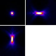
A: Bead (linear)
|
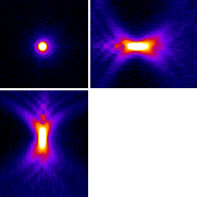
B: Bead (gamma)
|
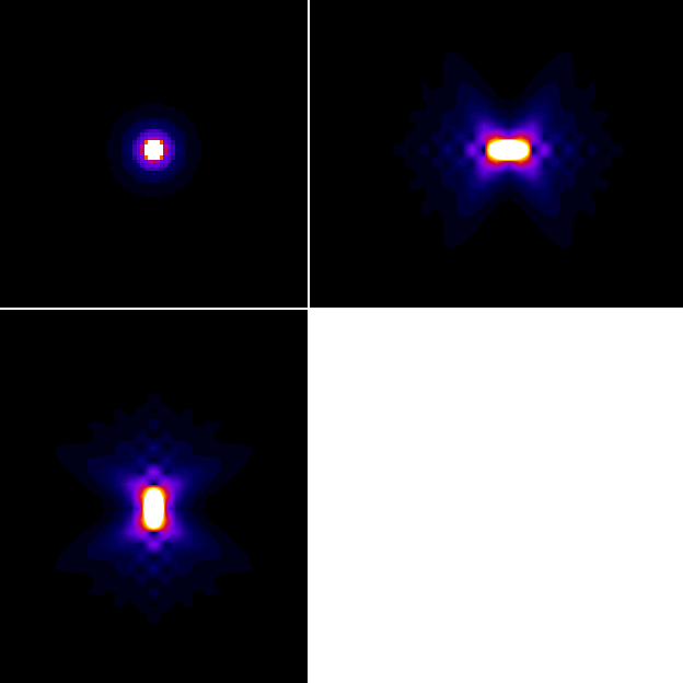
C: Theoretical PSF (linear)
|
Figure 3: PSFs for a widefield microscope. (A) and (B) are from z-stacks acquired of a small fluorescent bead, displayed using linear contrast and after applying a gamma transform to make fainter details easier to discern (see Manipulating individual pixels for more information). (C) shows a theoretical PSF for a similar microscope. It differs in appearance partly because the bead is not really an infinitesimally small point, and partly because the real microscope’s objective lens is less than perfect. Nevertheless, the overall shapes are similar.
In & out of focus
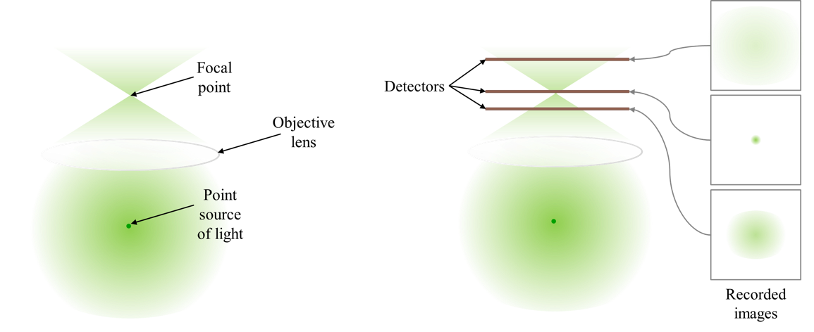
|
Figure 4: Simplified diagram to help visualize how a light-emitting point would be imaged using a widefield microscope. Some of the light originating from the point is captured by a lens. If you imagine the light then being directed towards a focal point, this leads to an hourglass shape. If a detector is placed close to the focal point, the spot-like image formed by the light striking the detector would be small and bright. However, if the detector were positioned above or below this focal plane, the intensity of the spot would decrease and its size would increase.
The appearance of interference
Figure 4 is quite limited in what it shows: it does not begin to explain the extra patterns of the PSF, which appear on each 2D plane as concentric rings (Figure 5), nor why the PSF does not shrink to a single point in the focal plane. These factors relate to the interference of light waves. While it is important to know that the rings occur – if only to avoid ever misinterpreting them as extra ring-like structures being really present in a sample – they have limited influence upon any analysis because the central region of the PSF is overwhelmingly brighter. Therefore for our purposes they can mostly be disregarded.

|

|

|

|

|

|

|

|

|

|
Figure 5: Ten slices from a z-stack acquired of a fluorescent bead, starting from above and moving down to the focal plane. The same linear contrast settings have been applied to each slice for easy comparison, although this causes the in-focus bead to appear saturated since otherwise the rings would not be visible at all. Because the image is (approximately) symmetrical along the z-axis, additional slices moving below the focal plane would appear similar.
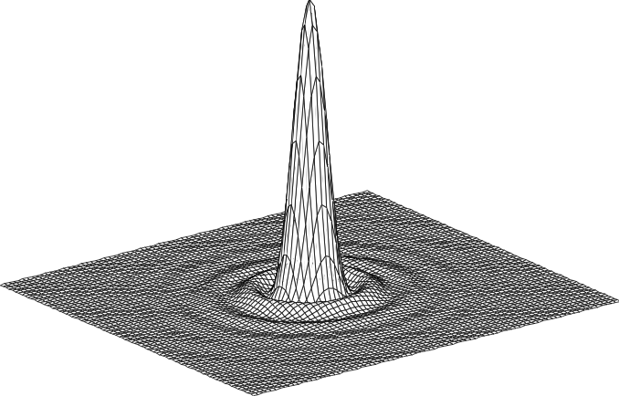
The Airy disk
Finally for this section, the PSF in the focal plane is important enough to deserve some attention, since we tend to want to measure things where they are most in-focus. This entire xy plane, including its interfering ripples, is called an Airy pattern, while the bright central part alone is the Airy disk (Figure 6). In the best possible case, when all the light in a 2D image comes from in-focus structures, it would already have been blurred by a filter that looks like this.

A: George Biddell Airy (1801–1892)
|

B: Airy pattern
|
C: Surface plot of Airy pattern
|
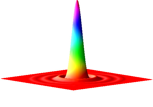
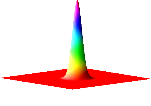
Figure 6: George Biddell Airy and the Airy pattern. (A) During his schooldays, Airy had been renowned for being skilled 'in the construction of peashooters and other such devices' (see http://www-history.mcs.st-and.ac.uk/Biographies/Airy.html). The rings surrounding the Airy disk have been likened to the ripples on a pond. Although the rings phenomenon was already known, Airy wrote the first theoretical treatment of it in 1835 (http://en.wikipedia.org/wiki/Airy_disk). (B) An Airy pattern, viewed as an image in which the contrast has been set to enhance the appearance of the outer rings surrounding the Airy disk. (C) A surface plot of an Airy pattern, which shows that the brightness is much higher within the central region when compared to the rings.
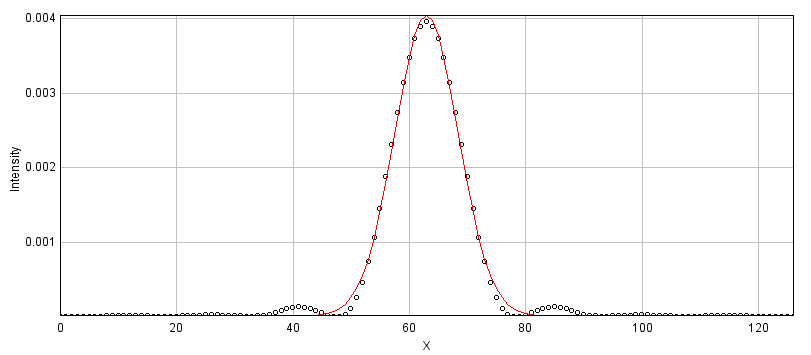
The Airy disk should look familiar. If we ignore the little interfering ripples around its edges, it can be very well approximated by a Gaussian function (Figure 7). Therefore the blur of a microscope in 2D is similar to applying a Gaussian filter, at least in the focal plane.
A: Airy disk
|
B: 2D Gaussian
|
C: Profile through the center of the Airy disk (black) and Gaussian fit (red)
|
Figure 7: Comparison of an Airy disk (taken from a theoretical PSF) and a Gaussian of a similar size, using two psychedelic surface plots and a 1D cross-section. The Gaussian is a very close match to the Airy disk.
The size of the PSF
So much for appearances. To judge how the blurring will affect what we can see and measure, we need to know the size of the PSF – where smaller would be preferable.
The size requires some defining: the PSF actually continues indefinitely, but has extremely low intensity values when far from its center. One approach for characterizing the Airy disk size is to consider its radius as the distance from the center to the first minimum: the lowest point before the first of the outer ripples begins. This is is given by:
where is the light wavelength and NA is the numerical aperture of the objective lens[1].
A comparable measurement to between the center and first minimum along the z axis is:
where is the refractive index of the objective lens immersion medium (which is a value related to the speed of light through that medium).

|
A: NA = 0.8
|
B: NA = 1.0
|
C: NA = 1.2
|
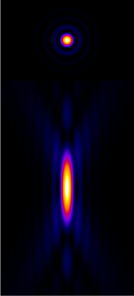
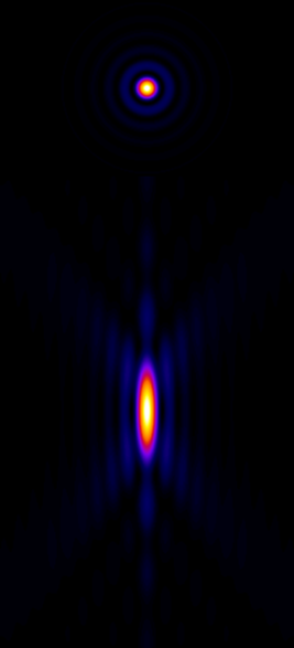
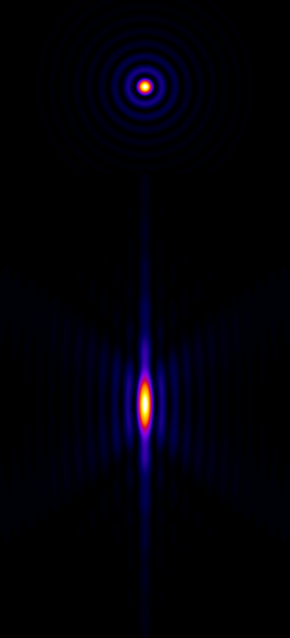
Figure 8: Examples of theoretical PSFs generated with different Numerical Apertures.
Numerical Aperture
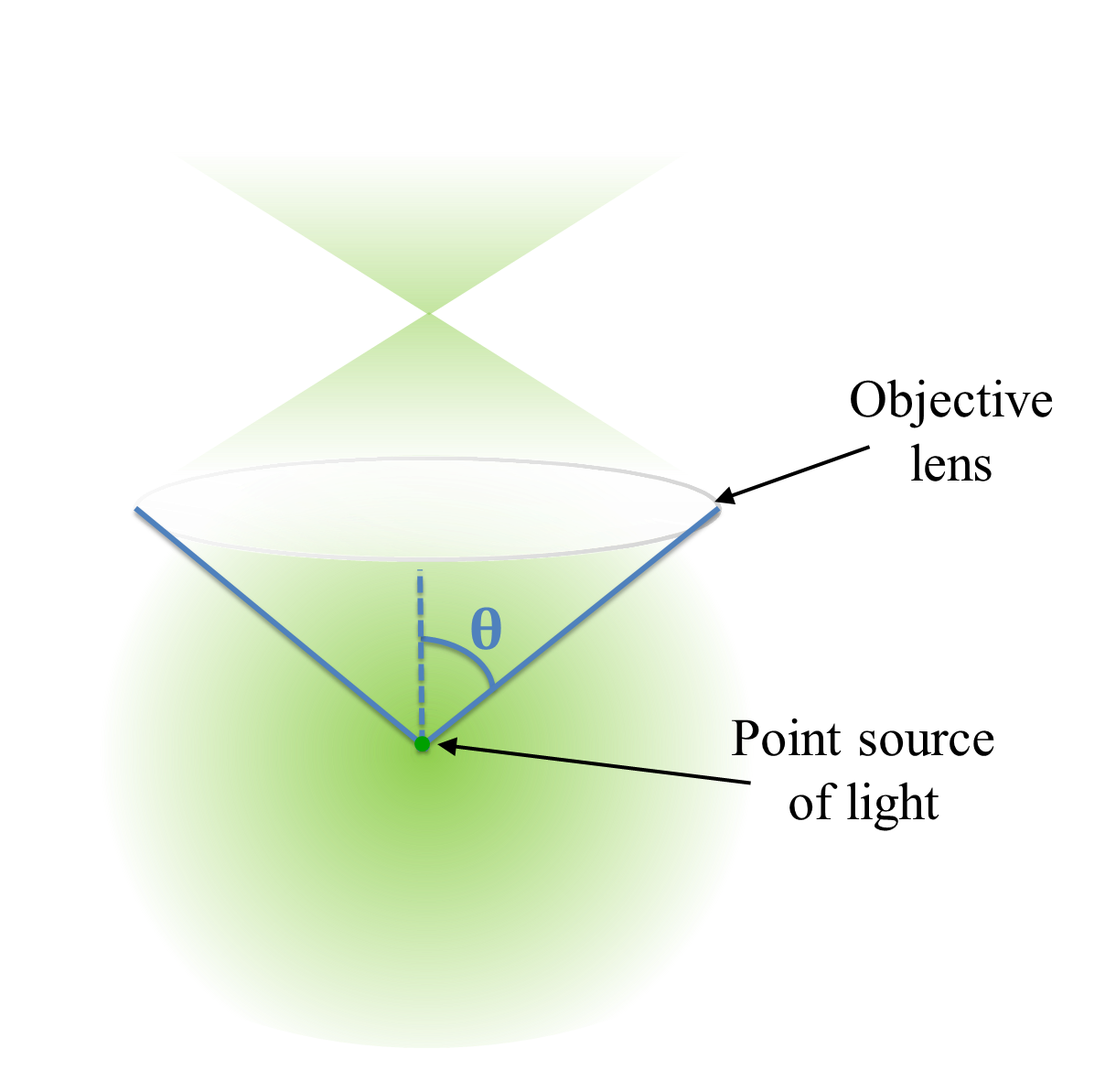
The equations for the PSF size show that if you can use an objective lens with a higher NA, you can potentially reduce blur in an image – especially along the z axis (Figure 8). Unfortunately, one soon reaches another limit in terms of what increasing the NA can achieve. This can be seen from the equation used to define it:
where is again the refractive index of the immersion medium and is the half-angle of the cone of light accepted by the objective (above). Because can never exceed 1, the NA can never exceed , which itself has fixed values (e.g. around 1.0 for air, 1.34 for water, or 1.5 for oil). High NA lenses can therefore reduce blur only to a limited degree.
An important additional consideration is that the highest NAs are possible when the immersion refractive index is high, but if this does not match the refractive index of the medium surrounding the sample we get spherical aberration. This is a phenomenon whereby the PSF becomes asymmetrical at increasing depth and the blur becomes weirder. Therefore, matching the refractive indices of the immersion and embedding media is often strongly preferable to using the highest NA objective available: it is usually better to have a larger PSF than a highly irregular one.
For an interactive tutorial on the effect of using different NAs, see http://www.microscopyu.com/tutorials/java/imageformation/airyna/index.html
Spatial resolution
Spatial resolution is concerned with how close two structures can be while they are still distinguishable. This is a somewhat subjective and fuzzy idea, but one way to define it is by the Rayleigh Criterion, according to which two equally bright spots are said to be resolved (i.e. distinguishable) if they are separated by the distances calculated in the lateral and axial equations above. If the spots are closer than this, they are likely to be seen as one. In the in-focus plane, this is illustrated in Figure 9.

|

|

|
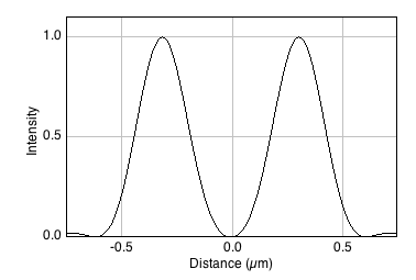
A: 2 disk radii separation
|
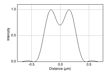
B: 1 disk radius separation
|
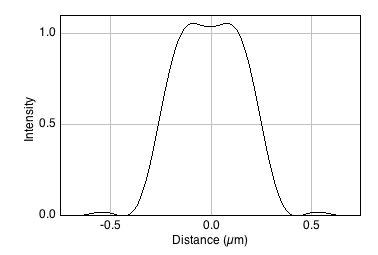
C: 0.8 disk radii separation
|
Figure 9: Airy patterns separated by different distances, defined in terms of Airy disk radii. The top row contains the patterns themselves, while the bottom row shows fluorescence intensity profiles computed across the centers of the patterns. Two distinct spots are clearly visible whenever separated by at least one disk radius, and there is a dip apparent in the profile. However, if the separation is less than one radius, the contrast rapidly decreases until only one structure is apparent.
It should be kept in mind that the use of and in the Rayleigh criterion is somewhat arbitrary – and the effects of brightness differences, finite pixel sizes and noise further complicate the situation, so that in practice a greater distance may well be required for us to confidently distinguish structures. Nevertheless, the Rayleigh criterion is helpful to give some idea of the scale of distances involved, i.e. hundreds of nanometers when using visible light.
Measuring PSFs & small structures
Knowing that the Airy disk resembles a Gaussian function is extremely useful, because any time we see an Airy disk we can fit a 2D Gaussian to it. The parameters of the function will then tell us the Gaussian’s center exactly, which corresponds to where the fluorescing structure really is – admittedly not with complete accuracy, but potentially still beyond the accuracy of even the pixel size (noise is the real limitation). This idea is fundamental to single-molecule localization techniques, including those in super-resolution microscopes like STORM and PALM, but requires that PSFs are sufficiently well-spaced that they do not interfere with one another and thereby ruin the fitting.
In ImageJ, we can somewhat approximate this localization by drawing a line profile across the peak of a PSF and then running . There we can fit a 1D Gaussian function, for which the equation used is
is simply a background constant, tells you the peak amplitude (i.e. the maximum value of the Gaussian with the background subtracted), and gives the location of the peak along the profile line. But potentially the most useful parameter here is , which corresponds to the value of a Gaussian filter. So if you know this value for a PSF, you can approximate the same amount of blurring with a Gaussian filter. This may come in useful in Simulating image formation.
1. Note that this is the limit of the Airy disk size, and assumes that the system is free of any aberrations. In other words, this is the best that we can hope for: the Airy disk cannot be made smaller simply by better focusing, although it could easily be made worse by a less-than-perfect objective lens.